Free Statistics
of Irreproducible Research!
Description of Statistical Computation | |||||||||||||||||||||||||||||||||||||||||||||||||||||||||||||||||||||||||||||||||
|---|---|---|---|---|---|---|---|---|---|---|---|---|---|---|---|---|---|---|---|---|---|---|---|---|---|---|---|---|---|---|---|---|---|---|---|---|---|---|---|---|---|---|---|---|---|---|---|---|---|---|---|---|---|---|---|---|---|---|---|---|---|---|---|---|---|---|---|---|---|---|---|---|---|---|---|---|---|---|---|---|---|
| Author's title | |||||||||||||||||||||||||||||||||||||||||||||||||||||||||||||||||||||||||||||||||
| Author | *Unverified author* | ||||||||||||||||||||||||||||||||||||||||||||||||||||||||||||||||||||||||||||||||
| R Software Module | rwasp_bootstrapplot.wasp | ||||||||||||||||||||||||||||||||||||||||||||||||||||||||||||||||||||||||||||||||
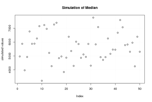
| Title produced by software | Blocked Bootstrap Plot - Central Tendency | ||||||||||||||||||||||||||||||||||||||||||||||||||||||||||||||||||||||||||||||||
| Date of computation | Sat, 08 May 2010 16:20:23 +0000 | ||||||||||||||||||||||||||||||||||||||||||||||||||||||||||||||||||||||||||||||||
| Cite this page as follows | Statistical Computations at FreeStatistics.org, Office for Research Development and Education, URL https://freestatistics.org/blog/index.php?v=date/2010/May/08/t127333565018rh2w5yt6v38og.htm/, Retrieved Sat, 05 Jul 2025 18:10:31 +0000 | ||||||||||||||||||||||||||||||||||||||||||||||||||||||||||||||||||||||||||||||||
| Statistical Computations at FreeStatistics.org, Office for Research Development and Education, URL https://freestatistics.org/blog/index.php?pk=75666, Retrieved Sat, 05 Jul 2025 18:10:31 +0000 | |||||||||||||||||||||||||||||||||||||||||||||||||||||||||||||||||||||||||||||||||
| QR Codes: | |||||||||||||||||||||||||||||||||||||||||||||||||||||||||||||||||||||||||||||||||
|
| |||||||||||||||||||||||||||||||||||||||||||||||||||||||||||||||||||||||||||||||||
| Original text written by user: | |||||||||||||||||||||||||||||||||||||||||||||||||||||||||||||||||||||||||||||||||
| IsPrivate? | No (this computation is public) | ||||||||||||||||||||||||||||||||||||||||||||||||||||||||||||||||||||||||||||||||
| User-defined keywords | KDGP2W32 | ||||||||||||||||||||||||||||||||||||||||||||||||||||||||||||||||||||||||||||||||
| Estimated Impact | 293 | ||||||||||||||||||||||||||||||||||||||||||||||||||||||||||||||||||||||||||||||||
Tree of Dependent Computations | |||||||||||||||||||||||||||||||||||||||||||||||||||||||||||||||||||||||||||||||||
| Family? (F = Feedback message, R = changed R code, M = changed R Module, P = changed Parameters, D = changed Data) | |||||||||||||||||||||||||||||||||||||||||||||||||||||||||||||||||||||||||||||||||
| - [Bootstrap Plot - Central Tendency] [] [2010-05-08 15:45:44] [c6ebbe7a5fe9990667cad80722534846] - P [Bootstrap Plot - Central Tendency] [] [2010-05-08 15:50:00] [c6ebbe7a5fe9990667cad80722534846] - RMPD [Blocked Bootstrap Plot - Central Tendency] [] [2010-05-08 16:20:23] [34252ed26d999a27212450e9b83760c6] [Current] - PD [Blocked Bootstrap Plot - Central Tendency] [] [2010-05-08 16:23:17] [c6ebbe7a5fe9990667cad80722534846] | |||||||||||||||||||||||||||||||||||||||||||||||||||||||||||||||||||||||||||||||||
| Feedback Forum | |||||||||||||||||||||||||||||||||||||||||||||||||||||||||||||||||||||||||||||||||
Post a new message | |||||||||||||||||||||||||||||||||||||||||||||||||||||||||||||||||||||||||||||||||
Dataset | |||||||||||||||||||||||||||||||||||||||||||||||||||||||||||||||||||||||||||||||||
| Dataseries X: | |||||||||||||||||||||||||||||||||||||||||||||||||||||||||||||||||||||||||||||||||
1772,2 1769,5 1768 1794,8 1823,4 1856,9 1866,9 1869,8 1843,8 1837,1 1857,7 1840,3 1914,6 1972,9 2050,1 2086,2 2112,5 2147,6 2190,4 2194,1 2216,2 2218,6 2233,5 2307,2 2350,4 2368,2 2353,8 2316,5 2305,5 2308,4 2334,4 2381,2 2449,7 2490,3 2523,5 2537,6 2526,1 2545,9 2542,7 2584,3 2600,2 2593,9 2618,9 2591,3 2521,2 2536,6 2596,1 2656,6 2710,3 2778,8 2775,5 2785,2 2847,7 2834,4 2839 2802,6 2819,3 2872 2918,4 2977,8 3031,2 3064,7 3093 3100,6 3141,1 3180,4 3240,3 3265 3338,2 3376,6 3422,5 3432 3516,3 3564 3636,3 3724 3815,4 3828,1 3853,3 3884,5 3918,7 3919,6 3950,8 3981 4063 4132 4160,3 4178,3 4244,1 4256,5 4283,4 4263,3 4256,6 4264,3 4302,3 4256,6 4374 4398,8 4433,9 4446,3 4525,8 4633,1 4677,5 4754,5 4876,2 4932,6 4906,3 4953,1 4909,6 4922,2 4873,5 4854,3 4795,3 4831,9 4913,3 4977,5 5090,7 5128,9 5154,1 5191,5 5251,8 5356,1 5451,9 5450,8 5469,4 5684,6 5740,3 5816,2 5825,9 5831,4 5873,3 5889,5 5908,5 5787,4 5776,6 5883,5 6005,7 5957,8 6030,2 5955,1 5857,3 5889,1 5866,4 5871 5944 6077,6 6197,5 6325,6 6448,3 6559,6 6623,3 6677,3 6740,3 6797,3 6903,5 6955,9 7022,8 7051 7119 7153,4 7193 7269,5 7332,6 7458 7496,6 7592,9 7632,1 7734 7806,6 7865 7927,4 7944,7 8027,7 8059,6 8059,5 7988,9 7950,2 8003,8 8037,5 8069 8157,6 8244,3 8329,4 8417 8432,5 8486,4 8531,1 8643,8 8727,9 8847,3 8904,3 9003,2 9025,3 9044,7 9120,7 9184,3 9247,2 9407,1 9488,9 9592,5 9666,2 9809,6 9932,7 10008,9 10103,4 10194,3 10328,8 10507,6 10601,2 10684 10819,9 11014,3 11043 11258,5 11267,9 11334,5 11297,2 11371,3 11340,1 11380,1 11477,9 11538,8 11596,4 11598,8 11645,8 11738,7 11935,5 12042,8 12127,6 12213,8 12303,5 12410,3 12534,1 12587,5 12683,2 12748,7 12915,9 12962,5 12965,9 13060,7 13099,9 13204 13321,1 13391,2 13366,9 13415,3 13324,6 13141,9 12925,4 12901,5 12973 13155 | |||||||||||||||||||||||||||||||||||||||||||||||||||||||||||||||||||||||||||||||||
Tables (Output of Computation) | |||||||||||||||||||||||||||||||||||||||||||||||||||||||||||||||||||||||||||||||||
| |||||||||||||||||||||||||||||||||||||||||||||||||||||||||||||||||||||||||||||||||
Figures (Output of Computation) | |||||||||||||||||||||||||||||||||||||||||||||||||||||||||||||||||||||||||||||||||
Input Parameters & R Code | |||||||||||||||||||||||||||||||||||||||||||||||||||||||||||||||||||||||||||||||||
| Parameters (Session): | |||||||||||||||||||||||||||||||||||||||||||||||||||||||||||||||||||||||||||||||||
| par1 = 50 ; par2 = 4 ; | |||||||||||||||||||||||||||||||||||||||||||||||||||||||||||||||||||||||||||||||||
| Parameters (R input): | |||||||||||||||||||||||||||||||||||||||||||||||||||||||||||||||||||||||||||||||||
| par1 = 50 ; par2 = 4 ; | |||||||||||||||||||||||||||||||||||||||||||||||||||||||||||||||||||||||||||||||||
| R code (references can be found in the software module): | |||||||||||||||||||||||||||||||||||||||||||||||||||||||||||||||||||||||||||||||||
par1 <- as.numeric(par1) | |||||||||||||||||||||||||||||||||||||||||||||||||||||||||||||||||||||||||||||||||