Free Statistics
of Irreproducible Research!
Description of Statistical Computation | |||||||||||||||||||||
|---|---|---|---|---|---|---|---|---|---|---|---|---|---|---|---|---|---|---|---|---|---|
| Author's title | |||||||||||||||||||||
| Author | *Unverified author* | ||||||||||||||||||||
| R Software Module | rwasp_meanplot.wasp | ||||||||||||||||||||
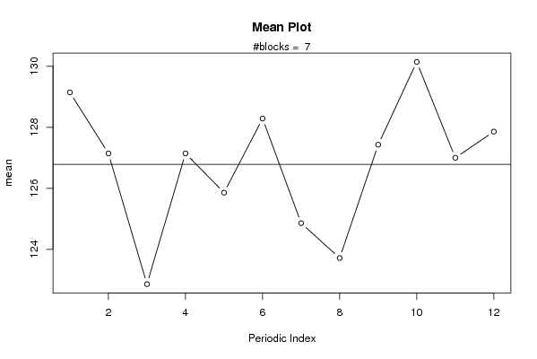
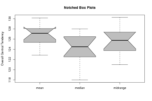
| Title produced by software | Mean Plot | ||||||||||||||||||||
| Date of computation | Thu, 29 Jul 2010 12:48:29 +0000 | ||||||||||||||||||||
| Cite this page as follows | Statistical Computations at FreeStatistics.org, Office for Research Development and Education, URL https://freestatistics.org/blog/index.php?v=date/2010/Jul/29/t1280407709mgb20m1qydrk35m.htm/, Retrieved Sun, 28 Apr 2024 21:00:43 +0000 | ||||||||||||||||||||
| Statistical Computations at FreeStatistics.org, Office for Research Development and Education, URL https://freestatistics.org/blog/index.php?pk=78176, Retrieved Sun, 28 Apr 2024 21:00:43 +0000 | |||||||||||||||||||||
| QR Codes: | |||||||||||||||||||||
|
| |||||||||||||||||||||
| Original text written by user: | |||||||||||||||||||||
| IsPrivate? | No (this computation is public) | ||||||||||||||||||||
| User-defined keywords | Hoes Isabelle | ||||||||||||||||||||
| Estimated Impact | 161 | ||||||||||||||||||||
Tree of Dependent Computations | |||||||||||||||||||||
| Family? (F = Feedback message, R = changed R code, M = changed R Module, P = changed Parameters, D = changed Data) | |||||||||||||||||||||
| - [Harrell-Davis Quantiles] [TIJDREEKS A - STA...] [2010-07-26 14:12:53] [0b48553e7c30a6637a1907066e9be3d4] - RMPD [Mean Plot] [TIJDREEKS B - STA...] [2010-07-29 12:48:29] [35611de12c9fa8a4a915f3548e0dcd01] [Current] | |||||||||||||||||||||
| Feedback Forum | |||||||||||||||||||||
Post a new message | |||||||||||||||||||||
Dataset | |||||||||||||||||||||
| Dataseries X: | |||||||||||||||||||||
158 157 156 154 152 151 152 154 155 155 156 158 156 152 145 141 140 145 143 141 144 139 141 142 141 132 122 122 127 128 122 123 128 128 128 129 124 121 109 110 107 107 104 110 114 118 117 122 113 106 102 111 106 110 105 104 106 110 107 111 101 105 108 124 122 128 124 121 125 134 126 126 111 117 118 128 127 129 124 113 120 127 114 107 | |||||||||||||||||||||
Tables (Output of Computation) | |||||||||||||||||||||
| |||||||||||||||||||||
Figures (Output of Computation) | |||||||||||||||||||||
Input Parameters & R Code | |||||||||||||||||||||
| Parameters (Session): | |||||||||||||||||||||
| par1 = 12 ; | |||||||||||||||||||||
| Parameters (R input): | |||||||||||||||||||||
| par1 = 12 ; | |||||||||||||||||||||
| R code (references can be found in the software module): | |||||||||||||||||||||
par1 <- as.numeric(par1) | |||||||||||||||||||||