Free Statistics
of Irreproducible Research!
Description of Statistical Computation | |||||||||||||||||||||
|---|---|---|---|---|---|---|---|---|---|---|---|---|---|---|---|---|---|---|---|---|---|
| Author's title | |||||||||||||||||||||
| Author | *Unverified author* | ||||||||||||||||||||
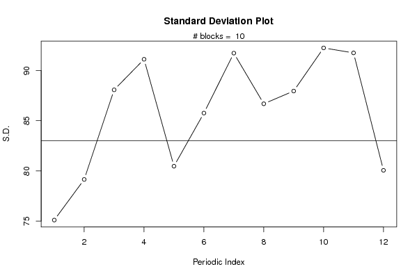
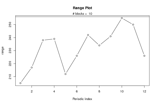
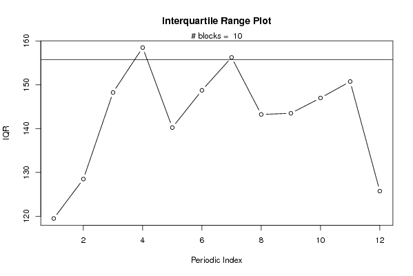
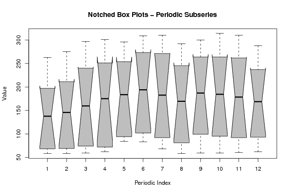
| R Software Module | rwasp_sdplot.wasp | ||||||||||||||||||||
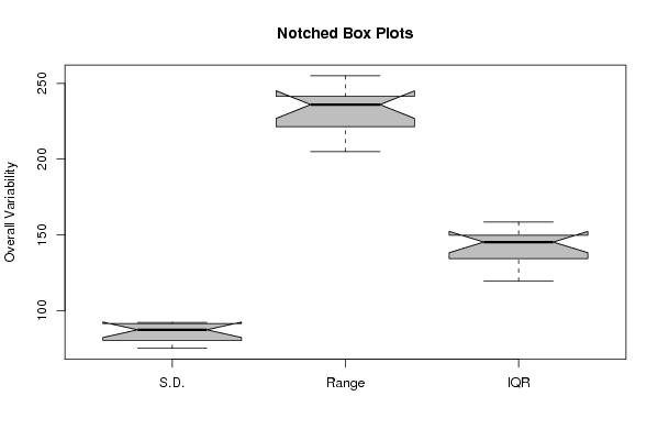
| Title produced by software | Standard Deviation Plot | ||||||||||||||||||||
| Date of computation | Thu, 01 Jul 2010 17:38:08 +0000 | ||||||||||||||||||||
| Cite this page as follows | Statistical Computations at FreeStatistics.org, Office for Research Development and Education, URL https://freestatistics.org/blog/index.php?v=date/2010/Jul/01/t1278005922rcyrkzpzkzimj8p.htm/, Retrieved Sat, 04 May 2024 03:45:18 +0000 | ||||||||||||||||||||
| Statistical Computations at FreeStatistics.org, Office for Research Development and Education, URL https://freestatistics.org/blog/index.php?pk=77903, Retrieved Sat, 04 May 2024 03:45:18 +0000 | |||||||||||||||||||||
| QR Codes: | |||||||||||||||||||||
|
| |||||||||||||||||||||
| Original text written by user: | |||||||||||||||||||||
| IsPrivate? | No (this computation is public) | ||||||||||||||||||||
| User-defined keywords | thomas talboom | ||||||||||||||||||||
| Estimated Impact | 184 | ||||||||||||||||||||
Tree of Dependent Computations | |||||||||||||||||||||
| Family? (F = Feedback message, R = changed R code, M = changed R Module, P = changed Parameters, D = changed Data) | |||||||||||||||||||||
| - [Harrell-Davis Quantiles] [percentielen] [2010-07-01 11:45:42] [b6623a0531b43a362887826f077b4445] - RMP [Standard Deviation Plot] [spreidingsgrafieken] [2010-07-01 17:38:08] [58d9ccda37eeb031a0ffa1e9ea016ece] [Current] | |||||||||||||||||||||
| Feedback Forum | |||||||||||||||||||||
Post a new message | |||||||||||||||||||||
Dataset | |||||||||||||||||||||
| Dataseries X: | |||||||||||||||||||||
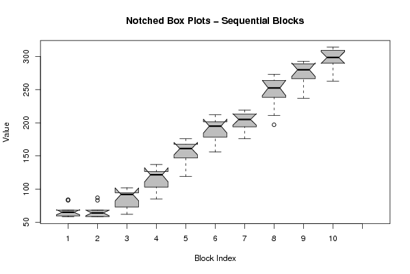
68 67 66 64 84 83 68 58 59 59 60 62 58 58 59 62 87 83 68 58 68 63 65 68 62 69 74 72 94 102 92 81 99 95 92 93 85 92 99 107 125 137 125 115 135 128 120 123 119 128 139 155 164 176 162 155 174 171 162 160 156 163 180 195 203 212 203 184 200 198 195 177 176 180 194 204 206 219 213 196 214 209 213 194 197 211 240 251 254 273 271 245 264 264 262 237 237 251 272 282 278 291 293 271 284 290 288 262 263 275 297 301 296 309 310 292 300 314 310 288 | |||||||||||||||||||||
Tables (Output of Computation) | |||||||||||||||||||||
| |||||||||||||||||||||
Figures (Output of Computation) | |||||||||||||||||||||
Input Parameters & R Code | |||||||||||||||||||||
| Parameters (Session): | |||||||||||||||||||||
| par1 = 0.01 ; par2 = 0.99 ; par3 = 0.1 ; | |||||||||||||||||||||
| Parameters (R input): | |||||||||||||||||||||
| par1 = 12 ; | |||||||||||||||||||||
| R code (references can be found in the software module): | |||||||||||||||||||||
par1 <- as.numeric(par1) | |||||||||||||||||||||