Repository of Reproducible Computations

Free Statistics

of Irreproducible Research!

Author's title

Author

*Unverified author*

R Software Module

rwasp_autocorrelation.wasp

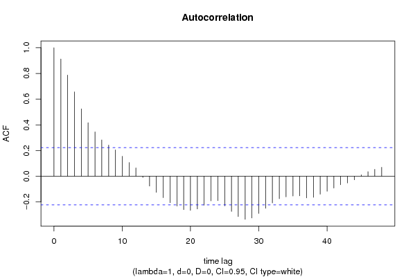
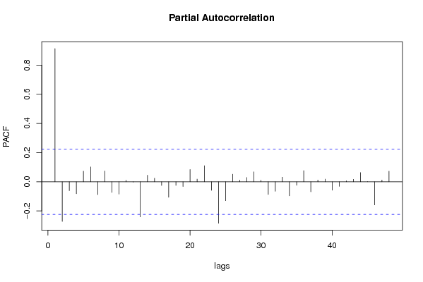
Title produced by software

(Partial) Autocorrelation Function

Date of computation

Mon, 25 Jan 2010 07:02:55 -0700

Cite this page as follows

Statistical Computations at FreeStatistics.org, Office for Research Development and Education, URL https://freestatistics.org/blog/index.php?v=date/2010/Jan/25/t1264428251vsyx7slxotcysn8.htm/, Retrieved Mon, 06 May 2024 04:47:06 +0000

Statistical Computations at FreeStatistics.org, Office for Research Development and Education, URL https://freestatistics.org/blog/index.php?pk=72447, Retrieved Mon, 06 May 2024 04:47:06 +0000

QR Codes:

Paste this QR Code to cite your computation.

Original text written by user:

IsPrivate?

No (this computation is public)

User-defined keywords

KDGP2W21

Estimated Impact

152

Family? (F = Feedback message, R = changed R code, M = changed R Module, P = changed Parameters, D = changed Data)

-     [(Partial) Autocorrelation Function] [Autocorrelation F...] [2010-01-25 13:50:04] [830dacb160eeaee72e8ff2204da365bc]
-    D    [(Partial) Autocorrelation Function] [Autocorrelation F...] [2010-01-25 14:02:55] [3588db8f96a346e7899895ad48978494] [Current]
-   PD      [(Partial) Autocorrelation Function] [degree of non-sea...] [2010-01-25 14:08:28] [830dacb160eeaee72e8ff2204da365bc] 
- RMPD      [Bootstrap Plot - Central Tendency] [Bootstrap Plot] [2010-01-25 14:33:20] [830dacb160eeaee72e8ff2204da365bc] 
- RMP       [Blocked Bootstrap Plot - Central Tendency] [Bootstrap Plot Porto] [2010-01-25 15:18:03] [830dacb160eeaee72e8ff2204da365bc] 
- RMPD      [Variability] [Variability Studi...] [2010-01-25 15:41:59] [830dacb160eeaee72e8ff2204da365bc] 
- RMPD      [Standard Deviation Plot] [spreidingsgrafiek...] [2010-01-25 15:50:06] [830dacb160eeaee72e8ff2204da365bc] 
- RMPD      [Standard Deviation-Mean Plot] [spreidings- en ge...] [2010-01-25 16:03:08] [830dacb160eeaee72e8ff2204da365bc] 
- RMP       [Variability] [Variability Porto] [2010-01-25 16:10:40] [830dacb160eeaee72e8ff2204da365bc] 
- RMP       [Standard Deviation Plot] [spreidingsgrafiek...] [2010-01-25 16:16:30] [830dacb160eeaee72e8ff2204da365bc] 
- RMP       [Standard Deviation-Mean Plot] [spreidings- en ge...] [2010-01-25 16:25:42] [830dacb160eeaee72e8ff2204da365bc] 
- RMPD      [Classical Decomposition] [decompositie pers...] [2010-01-25 17:04:08] [830dacb160eeaee72e8ff2204da365bc] 
- RMPD      [Classical Decomposition] [decompositie porto] [2010-01-25 17:20:25] [830dacb160eeaee72e8ff2204da365bc] 
- RMPD      [Exponential Smoothing] [Exponential smoot...] [2010-01-25 17:43:41] [830dacb160eeaee72e8ff2204da365bc] 
- RMP       [Exponential Smoothing] [Exponential smoot...] [2010-01-25 17:48:59] [830dacb160eeaee72e8ff2204da365bc] 

Feedback Forum

Post a new message

Dataseries X:

Download CSV

Histogram

Boxplots

8,2
8,21
8,22
8,2
8,18
8,2
8,19
8,24
8,31
8,27
8,36
8,32
8,29
8,27
8,27
8,43
8,46
8,48
8,46
8,46
8,43
8,4
8,38
8,3
8,39
8,53
8,52
8,54
8,62
8,52
8,49
8,44
8,31
8,26
8,21
8,03
7,89
7,83
7,85
7,84
7,88
8,01
8,08
8,11
8,11
8,07
8,06
7,95
7,95
8,07
8,17
8,21
8,2
8,19
8,18
8,16
8,17
8,17
8,19
8,01
8,04
8,13
8,14
8,17
8,25
8,27
8,27
8,26
8,24
8,21
8,25
8,06
8,16
8,32
8,43
8,39
8,41

Summary of computational transaction
Raw Input	view raw input (R code)
Raw Output	view raw output of R engine
Computing time	3 seconds
R Server	'Gwilym Jenkins' @ 72.249.127.135

\begin{tabular}{lllllllll}
\hline
Summary of computational transaction \tabularnewline
Raw Input & view raw input (R code)  \tabularnewline
Raw Output & view raw output of R engine  \tabularnewline
Computing time & 3 seconds \tabularnewline
R Server & 'Gwilym Jenkins' @ 72.249.127.135 \tabularnewline
\hline
\end{tabular}
%Source: https://freestatistics.org/blog/index.php?pk=72447&T=0

[TABLE]
[ROW][C]Summary of computational transaction[/C][/ROW]
[ROW][C]Raw Input[/C][C]view raw input (R code) [/C][/ROW]
[ROW][C]Raw Output[/C][C]view raw output of R engine [/C][/ROW]
[ROW][C]Computing time[/C][C]3 seconds[/C][/ROW]
[ROW][C]R Server[/C][C]'Gwilym Jenkins' @ 72.249.127.135[/C][/ROW]
[/TABLE]
Source: https://freestatistics.org/blog/index.php?pk=72447&T=0

Globally Unique Identifier (entire table): ba.freestatistics.org/blog/index.php?pk=72447&T=0

As an alternative you can also use a QR Code:

The GUIDs for individual cells are displayed in the table below:

Summary of computational transaction
Raw Input	view raw input (R code)
Raw Output	view raw output of R engine
Computing time	3 seconds
R Server	'Gwilym Jenkins' @ 72.249.127.135

Autocorrelation Function
Time lag k	ACF(k)	T-STAT	P-value
1	0.912579	8.0078	0
2	0.787304	6.9086	0
3	0.656208	5.7582	0
4	0.524049	4.5985	8e-06
5	0.416222	3.6523	0.000236
6	0.345233	3.0294	0.001667
7	0.282602	2.4798	0.007665
8	0.242	2.1235	0.01846
9	0.204705	1.7963	0.038186
10	0.154914	1.3594	0.089
11	0.106846	0.9376	0.175699
12	0.064851	0.5691	0.285483
13	-0.009756	-0.0856	0.465999
14	-0.077009	-0.6758	0.25061
15	-0.125987	-1.1055	0.136185
16	-0.167195	-1.4671	0.073206
17	-0.205832	-1.8062	0.0374
18	-0.232144	-2.0371	0.022541
19	-0.260262	-2.2838	0.01257
20	-0.265898	-2.3332	0.011124
21	-0.255424	-2.2413	0.013942
22	-0.225801	-1.9814	0.025559
23	-0.191722	-1.6824	0.048275
24	-0.190302	-1.6699	0.049501
25	-0.230631	-2.0238	0.023231
26	-0.274308	-2.407	0.009239
27	-0.31383	-2.7538	0.003672
28	-0.335292	-2.9422	0.002152
29	-0.325322	-2.8547	0.002766
30	-0.289385	-2.5393	0.006561
31	-0.249978	-2.1935	0.015643
32	-0.208329	-1.8281	0.035705
33	-0.175439	-1.5395	0.063894
34	-0.16113	-1.4139	0.08071
35	-0.15412	-1.3524	0.090104
36	-0.152606	-1.3391	0.092237
37	-0.168833	-1.4815	0.071277
38	-0.164464	-1.4432	0.076515
39	-0.139852	-1.2272	0.111743
40	-0.117078	-1.0274	0.153734
41	-0.092539	-0.812	0.20964
42	-0.066457	-0.5832	0.280747
43	-0.052451	-0.4603	0.323314
44	-0.028439	-0.2496	0.401799
45	0.011071	0.0972	0.461429
46	0.035481	0.3113	0.37819
47	0.053068	0.4657	0.321383
48	0.069393	0.6089	0.272185

\begin{tabular}{lllllllll}
\hline
Autocorrelation Function \tabularnewline
Time lag k & ACF(k) & T-STAT & P-value \tabularnewline
1 & 0.912579 & 8.0078 & 0 \tabularnewline
2 & 0.787304 & 6.9086 & 0 \tabularnewline
3 & 0.656208 & 5.7582 & 0 \tabularnewline
4 & 0.524049 & 4.5985 & 8e-06 \tabularnewline
5 & 0.416222 & 3.6523 & 0.000236 \tabularnewline
6 & 0.345233 & 3.0294 & 0.001667 \tabularnewline
7 & 0.282602 & 2.4798 & 0.007665 \tabularnewline
8 & 0.242 & 2.1235 & 0.01846 \tabularnewline
9 & 0.204705 & 1.7963 & 0.038186 \tabularnewline
10 & 0.154914 & 1.3594 & 0.089 \tabularnewline
11 & 0.106846 & 0.9376 & 0.175699 \tabularnewline
12 & 0.064851 & 0.5691 & 0.285483 \tabularnewline
13 & -0.009756 & -0.0856 & 0.465999 \tabularnewline
14 & -0.077009 & -0.6758 & 0.25061 \tabularnewline
15 & -0.125987 & -1.1055 & 0.136185 \tabularnewline
16 & -0.167195 & -1.4671 & 0.073206 \tabularnewline
17 & -0.205832 & -1.8062 & 0.0374 \tabularnewline
18 & -0.232144 & -2.0371 & 0.022541 \tabularnewline
19 & -0.260262 & -2.2838 & 0.01257 \tabularnewline
20 & -0.265898 & -2.3332 & 0.011124 \tabularnewline
21 & -0.255424 & -2.2413 & 0.013942 \tabularnewline
22 & -0.225801 & -1.9814 & 0.025559 \tabularnewline
23 & -0.191722 & -1.6824 & 0.048275 \tabularnewline
24 & -0.190302 & -1.6699 & 0.049501 \tabularnewline
25 & -0.230631 & -2.0238 & 0.023231 \tabularnewline
26 & -0.274308 & -2.407 & 0.009239 \tabularnewline
27 & -0.31383 & -2.7538 & 0.003672 \tabularnewline
28 & -0.335292 & -2.9422 & 0.002152 \tabularnewline
29 & -0.325322 & -2.8547 & 0.002766 \tabularnewline
30 & -0.289385 & -2.5393 & 0.006561 \tabularnewline
31 & -0.249978 & -2.1935 & 0.015643 \tabularnewline
32 & -0.208329 & -1.8281 & 0.035705 \tabularnewline
33 & -0.175439 & -1.5395 & 0.063894 \tabularnewline
34 & -0.16113 & -1.4139 & 0.08071 \tabularnewline
35 & -0.15412 & -1.3524 & 0.090104 \tabularnewline
36 & -0.152606 & -1.3391 & 0.092237 \tabularnewline
37 & -0.168833 & -1.4815 & 0.071277 \tabularnewline
38 & -0.164464 & -1.4432 & 0.076515 \tabularnewline
39 & -0.139852 & -1.2272 & 0.111743 \tabularnewline
40 & -0.117078 & -1.0274 & 0.153734 \tabularnewline
41 & -0.092539 & -0.812 & 0.20964 \tabularnewline
42 & -0.066457 & -0.5832 & 0.280747 \tabularnewline
43 & -0.052451 & -0.4603 & 0.323314 \tabularnewline
44 & -0.028439 & -0.2496 & 0.401799 \tabularnewline
45 & 0.011071 & 0.0972 & 0.461429 \tabularnewline
46 & 0.035481 & 0.3113 & 0.37819 \tabularnewline
47 & 0.053068 & 0.4657 & 0.321383 \tabularnewline
48 & 0.069393 & 0.6089 & 0.272185 \tabularnewline
\hline
\end{tabular}
%Source: https://freestatistics.org/blog/index.php?pk=72447&T=1

[TABLE]
[ROW][C]Autocorrelation Function[/C][/ROW]
[ROW][C]Time lag k[/C][C]ACF(k)[/C][C]T-STAT[/C][C]P-value[/C][/ROW]
[ROW][C]1[/C][C]0.912579[/C][C]8.0078[/C][C]0[/C][/ROW]
[ROW][C]2[/C][C]0.787304[/C][C]6.9086[/C][C]0[/C][/ROW]
[ROW][C]3[/C][C]0.656208[/C][C]5.7582[/C][C]0[/C][/ROW]
[ROW][C]4[/C][C]0.524049[/C][C]4.5985[/C][C]8e-06[/C][/ROW]
[ROW][C]5[/C][C]0.416222[/C][C]3.6523[/C][C]0.000236[/C][/ROW]
[ROW][C]6[/C][C]0.345233[/C][C]3.0294[/C][C]0.001667[/C][/ROW]
[ROW][C]7[/C][C]0.282602[/C][C]2.4798[/C][C]0.007665[/C][/ROW]
[ROW][C]8[/C][C]0.242[/C][C]2.1235[/C][C]0.01846[/C][/ROW]
[ROW][C]9[/C][C]0.204705[/C][C]1.7963[/C][C]0.038186[/C][/ROW]
[ROW][C]10[/C][C]0.154914[/C][C]1.3594[/C][C]0.089[/C][/ROW]
[ROW][C]11[/C][C]0.106846[/C][C]0.9376[/C][C]0.175699[/C][/ROW]
[ROW][C]12[/C][C]0.064851[/C][C]0.5691[/C][C]0.285483[/C][/ROW]
[ROW][C]13[/C][C]-0.009756[/C][C]-0.0856[/C][C]0.465999[/C][/ROW]
[ROW][C]14[/C][C]-0.077009[/C][C]-0.6758[/C][C]0.25061[/C][/ROW]
[ROW][C]15[/C][C]-0.125987[/C][C]-1.1055[/C][C]0.136185[/C][/ROW]
[ROW][C]16[/C][C]-0.167195[/C][C]-1.4671[/C][C]0.073206[/C][/ROW]
[ROW][C]17[/C][C]-0.205832[/C][C]-1.8062[/C][C]0.0374[/C][/ROW]
[ROW][C]18[/C][C]-0.232144[/C][C]-2.0371[/C][C]0.022541[/C][/ROW]
[ROW][C]19[/C][C]-0.260262[/C][C]-2.2838[/C][C]0.01257[/C][/ROW]
[ROW][C]20[/C][C]-0.265898[/C][C]-2.3332[/C][C]0.011124[/C][/ROW]
[ROW][C]21[/C][C]-0.255424[/C][C]-2.2413[/C][C]0.013942[/C][/ROW]
[ROW][C]22[/C][C]-0.225801[/C][C]-1.9814[/C][C]0.025559[/C][/ROW]
[ROW][C]23[/C][C]-0.191722[/C][C]-1.6824[/C][C]0.048275[/C][/ROW]
[ROW][C]24[/C][C]-0.190302[/C][C]-1.6699[/C][C]0.049501[/C][/ROW]
[ROW][C]25[/C][C]-0.230631[/C][C]-2.0238[/C][C]0.023231[/C][/ROW]
[ROW][C]26[/C][C]-0.274308[/C][C]-2.407[/C][C]0.009239[/C][/ROW]
[ROW][C]27[/C][C]-0.31383[/C][C]-2.7538[/C][C]0.003672[/C][/ROW]
[ROW][C]28[/C][C]-0.335292[/C][C]-2.9422[/C][C]0.002152[/C][/ROW]
[ROW][C]29[/C][C]-0.325322[/C][C]-2.8547[/C][C]0.002766[/C][/ROW]
[ROW][C]30[/C][C]-0.289385[/C][C]-2.5393[/C][C]0.006561[/C][/ROW]
[ROW][C]31[/C][C]-0.249978[/C][C]-2.1935[/C][C]0.015643[/C][/ROW]
[ROW][C]32[/C][C]-0.208329[/C][C]-1.8281[/C][C]0.035705[/C][/ROW]
[ROW][C]33[/C][C]-0.175439[/C][C]-1.5395[/C][C]0.063894[/C][/ROW]
[ROW][C]34[/C][C]-0.16113[/C][C]-1.4139[/C][C]0.08071[/C][/ROW]
[ROW][C]35[/C][C]-0.15412[/C][C]-1.3524[/C][C]0.090104[/C][/ROW]
[ROW][C]36[/C][C]-0.152606[/C][C]-1.3391[/C][C]0.092237[/C][/ROW]
[ROW][C]37[/C][C]-0.168833[/C][C]-1.4815[/C][C]0.071277[/C][/ROW]
[ROW][C]38[/C][C]-0.164464[/C][C]-1.4432[/C][C]0.076515[/C][/ROW]
[ROW][C]39[/C][C]-0.139852[/C][C]-1.2272[/C][C]0.111743[/C][/ROW]
[ROW][C]40[/C][C]-0.117078[/C][C]-1.0274[/C][C]0.153734[/C][/ROW]
[ROW][C]41[/C][C]-0.092539[/C][C]-0.812[/C][C]0.20964[/C][/ROW]
[ROW][C]42[/C][C]-0.066457[/C][C]-0.5832[/C][C]0.280747[/C][/ROW]
[ROW][C]43[/C][C]-0.052451[/C][C]-0.4603[/C][C]0.323314[/C][/ROW]
[ROW][C]44[/C][C]-0.028439[/C][C]-0.2496[/C][C]0.401799[/C][/ROW]
[ROW][C]45[/C][C]0.011071[/C][C]0.0972[/C][C]0.461429[/C][/ROW]
[ROW][C]46[/C][C]0.035481[/C][C]0.3113[/C][C]0.37819[/C][/ROW]
[ROW][C]47[/C][C]0.053068[/C][C]0.4657[/C][C]0.321383[/C][/ROW]
[ROW][C]48[/C][C]0.069393[/C][C]0.6089[/C][C]0.272185[/C][/ROW]
[/TABLE]
Source: https://freestatistics.org/blog/index.php?pk=72447&T=1

Globally Unique Identifier (entire table): ba.freestatistics.org/blog/index.php?pk=72447&T=1

As an alternative you can also use a QR Code:

The GUIDs for individual cells are displayed in the table below:

Autocorrelation Function
Time lag k	ACF(k)	T-STAT	P-value
1	0.912579	8.0078	0
2	0.787304	6.9086	0
3	0.656208	5.7582	0
4	0.524049	4.5985	8e-06
5	0.416222	3.6523	0.000236
6	0.345233	3.0294	0.001667
7	0.282602	2.4798	0.007665
8	0.242	2.1235	0.01846
9	0.204705	1.7963	0.038186
10	0.154914	1.3594	0.089
11	0.106846	0.9376	0.175699
12	0.064851	0.5691	0.285483
13	-0.009756	-0.0856	0.465999
14	-0.077009	-0.6758	0.25061
15	-0.125987	-1.1055	0.136185
16	-0.167195	-1.4671	0.073206
17	-0.205832	-1.8062	0.0374
18	-0.232144	-2.0371	0.022541
19	-0.260262	-2.2838	0.01257
20	-0.265898	-2.3332	0.011124
21	-0.255424	-2.2413	0.013942
22	-0.225801	-1.9814	0.025559
23	-0.191722	-1.6824	0.048275
24	-0.190302	-1.6699	0.049501
25	-0.230631	-2.0238	0.023231
26	-0.274308	-2.407	0.009239
27	-0.31383	-2.7538	0.003672
28	-0.335292	-2.9422	0.002152
29	-0.325322	-2.8547	0.002766
30	-0.289385	-2.5393	0.006561
31	-0.249978	-2.1935	0.015643
32	-0.208329	-1.8281	0.035705
33	-0.175439	-1.5395	0.063894
34	-0.16113	-1.4139	0.08071
35	-0.15412	-1.3524	0.090104
36	-0.152606	-1.3391	0.092237
37	-0.168833	-1.4815	0.071277
38	-0.164464	-1.4432	0.076515
39	-0.139852	-1.2272	0.111743
40	-0.117078	-1.0274	0.153734
41	-0.092539	-0.812	0.20964
42	-0.066457	-0.5832	0.280747
43	-0.052451	-0.4603	0.323314
44	-0.028439	-0.2496	0.401799
45	0.011071	0.0972	0.461429
46	0.035481	0.3113	0.37819
47	0.053068	0.4657	0.321383
48	0.069393	0.6089	0.272185

Partial Autocorrelation Function
Time lag k	PACF(k)	T-STAT	P-value
1	0.912579	8.0078	0
2	-0.272102	-2.3877	0.009703
3	-0.06106	-0.5358	0.296821
4	-0.082293	-0.7221	0.236204
5	0.072701	0.6379	0.262701
6	0.101626	0.8918	0.187648
7	-0.088057	-0.7727	0.221034
8	0.073867	0.6482	0.259399
9	-0.073022	-0.6408	0.261789
10	-0.084734	-0.7435	0.22971
11	0.011086	0.0973	0.461378
12	-0.002248	-0.0197	0.492157
13	-0.240753	-2.1126	0.018938
14	0.044942	0.3944	0.3472
15	0.024464	0.2147	0.415296
16	-0.0252	-0.2211	0.412787
17	-0.106483	-0.9344	0.176512
18	-0.024617	-0.216	0.414776
19	-0.032905	-0.2887	0.386779
20	0.083718	0.7346	0.2324
21	0.018077	0.1586	0.43719
22	0.110011	0.9653	0.168697
23	-0.058904	-0.5169	0.303362
24	-0.284325	-2.4949	0.007369
25	-0.129872	-1.1396	0.128987
26	0.051635	0.4531	0.325877
27	0.01167	0.1024	0.459352
28	0.02913	0.2556	0.399464
29	0.067824	0.5952	0.276743
30	0.010778	0.0946	0.46245
31	-0.086755	-0.7613	0.224409
32	-0.065107	-0.5713	0.284725
33	0.031639	0.2776	0.39102
34	-0.096408	-0.846	0.200094
35	-0.024173	-0.2121	0.416288
36	0.075992	0.6668	0.253437
37	-0.068703	-0.6029	0.274186
38	0.012147	0.1066	0.457698
39	0.01839	0.1614	0.436113
40	-0.058227	-0.5109	0.305428
41	-0.03142	-0.2757	0.391756
42	0.006905	0.0606	0.475922
43	0.017004	0.1492	0.440888
44	0.062743	0.5506	0.291763
45	0.000367	0.0032	0.49872
46	-0.159015	-1.3953	0.083461
47	0.012155	0.1067	0.457667
48	0.072763	0.6385	0.262523

\begin{tabular}{lllllllll}
\hline
Partial Autocorrelation Function \tabularnewline
Time lag k & PACF(k) & T-STAT & P-value \tabularnewline
1 & 0.912579 & 8.0078 & 0 \tabularnewline
2 & -0.272102 & -2.3877 & 0.009703 \tabularnewline
3 & -0.06106 & -0.5358 & 0.296821 \tabularnewline
4 & -0.082293 & -0.7221 & 0.236204 \tabularnewline
5 & 0.072701 & 0.6379 & 0.262701 \tabularnewline
6 & 0.101626 & 0.8918 & 0.187648 \tabularnewline
7 & -0.088057 & -0.7727 & 0.221034 \tabularnewline
8 & 0.073867 & 0.6482 & 0.259399 \tabularnewline
9 & -0.073022 & -0.6408 & 0.261789 \tabularnewline
10 & -0.084734 & -0.7435 & 0.22971 \tabularnewline
11 & 0.011086 & 0.0973 & 0.461378 \tabularnewline
12 & -0.002248 & -0.0197 & 0.492157 \tabularnewline
13 & -0.240753 & -2.1126 & 0.018938 \tabularnewline
14 & 0.044942 & 0.3944 & 0.3472 \tabularnewline
15 & 0.024464 & 0.2147 & 0.415296 \tabularnewline
16 & -0.0252 & -0.2211 & 0.412787 \tabularnewline
17 & -0.106483 & -0.9344 & 0.176512 \tabularnewline
18 & -0.024617 & -0.216 & 0.414776 \tabularnewline
19 & -0.032905 & -0.2887 & 0.386779 \tabularnewline
20 & 0.083718 & 0.7346 & 0.2324 \tabularnewline
21 & 0.018077 & 0.1586 & 0.43719 \tabularnewline
22 & 0.110011 & 0.9653 & 0.168697 \tabularnewline
23 & -0.058904 & -0.5169 & 0.303362 \tabularnewline
24 & -0.284325 & -2.4949 & 0.007369 \tabularnewline
25 & -0.129872 & -1.1396 & 0.128987 \tabularnewline
26 & 0.051635 & 0.4531 & 0.325877 \tabularnewline
27 & 0.01167 & 0.1024 & 0.459352 \tabularnewline
28 & 0.02913 & 0.2556 & 0.399464 \tabularnewline
29 & 0.067824 & 0.5952 & 0.276743 \tabularnewline
30 & 0.010778 & 0.0946 & 0.46245 \tabularnewline
31 & -0.086755 & -0.7613 & 0.224409 \tabularnewline
32 & -0.065107 & -0.5713 & 0.284725 \tabularnewline
33 & 0.031639 & 0.2776 & 0.39102 \tabularnewline
34 & -0.096408 & -0.846 & 0.200094 \tabularnewline
35 & -0.024173 & -0.2121 & 0.416288 \tabularnewline
36 & 0.075992 & 0.6668 & 0.253437 \tabularnewline
37 & -0.068703 & -0.6029 & 0.274186 \tabularnewline
38 & 0.012147 & 0.1066 & 0.457698 \tabularnewline
39 & 0.01839 & 0.1614 & 0.436113 \tabularnewline
40 & -0.058227 & -0.5109 & 0.305428 \tabularnewline
41 & -0.03142 & -0.2757 & 0.391756 \tabularnewline
42 & 0.006905 & 0.0606 & 0.475922 \tabularnewline
43 & 0.017004 & 0.1492 & 0.440888 \tabularnewline
44 & 0.062743 & 0.5506 & 0.291763 \tabularnewline
45 & 0.000367 & 0.0032 & 0.49872 \tabularnewline
46 & -0.159015 & -1.3953 & 0.083461 \tabularnewline
47 & 0.012155 & 0.1067 & 0.457667 \tabularnewline
48 & 0.072763 & 0.6385 & 0.262523 \tabularnewline
\hline
\end{tabular}
%Source: https://freestatistics.org/blog/index.php?pk=72447&T=2

[TABLE]
[ROW][C]Partial Autocorrelation Function[/C][/ROW]
[ROW][C]Time lag k[/C][C]PACF(k)[/C][C]T-STAT[/C][C]P-value[/C][/ROW]
[ROW][C]1[/C][C]0.912579[/C][C]8.0078[/C][C]0[/C][/ROW]
[ROW][C]2[/C][C]-0.272102[/C][C]-2.3877[/C][C]0.009703[/C][/ROW]
[ROW][C]3[/C][C]-0.06106[/C][C]-0.5358[/C][C]0.296821[/C][/ROW]
[ROW][C]4[/C][C]-0.082293[/C][C]-0.7221[/C][C]0.236204[/C][/ROW]
[ROW][C]5[/C][C]0.072701[/C][C]0.6379[/C][C]0.262701[/C][/ROW]
[ROW][C]6[/C][C]0.101626[/C][C]0.8918[/C][C]0.187648[/C][/ROW]
[ROW][C]7[/C][C]-0.088057[/C][C]-0.7727[/C][C]0.221034[/C][/ROW]
[ROW][C]8[/C][C]0.073867[/C][C]0.6482[/C][C]0.259399[/C][/ROW]
[ROW][C]9[/C][C]-0.073022[/C][C]-0.6408[/C][C]0.261789[/C][/ROW]
[ROW][C]10[/C][C]-0.084734[/C][C]-0.7435[/C][C]0.22971[/C][/ROW]
[ROW][C]11[/C][C]0.011086[/C][C]0.0973[/C][C]0.461378[/C][/ROW]
[ROW][C]12[/C][C]-0.002248[/C][C]-0.0197[/C][C]0.492157[/C][/ROW]
[ROW][C]13[/C][C]-0.240753[/C][C]-2.1126[/C][C]0.018938[/C][/ROW]
[ROW][C]14[/C][C]0.044942[/C][C]0.3944[/C][C]0.3472[/C][/ROW]
[ROW][C]15[/C][C]0.024464[/C][C]0.2147[/C][C]0.415296[/C][/ROW]
[ROW][C]16[/C][C]-0.0252[/C][C]-0.2211[/C][C]0.412787[/C][/ROW]
[ROW][C]17[/C][C]-0.106483[/C][C]-0.9344[/C][C]0.176512[/C][/ROW]
[ROW][C]18[/C][C]-0.024617[/C][C]-0.216[/C][C]0.414776[/C][/ROW]
[ROW][C]19[/C][C]-0.032905[/C][C]-0.2887[/C][C]0.386779[/C][/ROW]
[ROW][C]20[/C][C]0.083718[/C][C]0.7346[/C][C]0.2324[/C][/ROW]
[ROW][C]21[/C][C]0.018077[/C][C]0.1586[/C][C]0.43719[/C][/ROW]
[ROW][C]22[/C][C]0.110011[/C][C]0.9653[/C][C]0.168697[/C][/ROW]
[ROW][C]23[/C][C]-0.058904[/C][C]-0.5169[/C][C]0.303362[/C][/ROW]
[ROW][C]24[/C][C]-0.284325[/C][C]-2.4949[/C][C]0.007369[/C][/ROW]
[ROW][C]25[/C][C]-0.129872[/C][C]-1.1396[/C][C]0.128987[/C][/ROW]
[ROW][C]26[/C][C]0.051635[/C][C]0.4531[/C][C]0.325877[/C][/ROW]
[ROW][C]27[/C][C]0.01167[/C][C]0.1024[/C][C]0.459352[/C][/ROW]
[ROW][C]28[/C][C]0.02913[/C][C]0.2556[/C][C]0.399464[/C][/ROW]
[ROW][C]29[/C][C]0.067824[/C][C]0.5952[/C][C]0.276743[/C][/ROW]
[ROW][C]30[/C][C]0.010778[/C][C]0.0946[/C][C]0.46245[/C][/ROW]
[ROW][C]31[/C][C]-0.086755[/C][C]-0.7613[/C][C]0.224409[/C][/ROW]
[ROW][C]32[/C][C]-0.065107[/C][C]-0.5713[/C][C]0.284725[/C][/ROW]
[ROW][C]33[/C][C]0.031639[/C][C]0.2776[/C][C]0.39102[/C][/ROW]
[ROW][C]34[/C][C]-0.096408[/C][C]-0.846[/C][C]0.200094[/C][/ROW]
[ROW][C]35[/C][C]-0.024173[/C][C]-0.2121[/C][C]0.416288[/C][/ROW]
[ROW][C]36[/C][C]0.075992[/C][C]0.6668[/C][C]0.253437[/C][/ROW]
[ROW][C]37[/C][C]-0.068703[/C][C]-0.6029[/C][C]0.274186[/C][/ROW]
[ROW][C]38[/C][C]0.012147[/C][C]0.1066[/C][C]0.457698[/C][/ROW]
[ROW][C]39[/C][C]0.01839[/C][C]0.1614[/C][C]0.436113[/C][/ROW]
[ROW][C]40[/C][C]-0.058227[/C][C]-0.5109[/C][C]0.305428[/C][/ROW]
[ROW][C]41[/C][C]-0.03142[/C][C]-0.2757[/C][C]0.391756[/C][/ROW]
[ROW][C]42[/C][C]0.006905[/C][C]0.0606[/C][C]0.475922[/C][/ROW]
[ROW][C]43[/C][C]0.017004[/C][C]0.1492[/C][C]0.440888[/C][/ROW]
[ROW][C]44[/C][C]0.062743[/C][C]0.5506[/C][C]0.291763[/C][/ROW]
[ROW][C]45[/C][C]0.000367[/C][C]0.0032[/C][C]0.49872[/C][/ROW]
[ROW][C]46[/C][C]-0.159015[/C][C]-1.3953[/C][C]0.083461[/C][/ROW]
[ROW][C]47[/C][C]0.012155[/C][C]0.1067[/C][C]0.457667[/C][/ROW]
[ROW][C]48[/C][C]0.072763[/C][C]0.6385[/C][C]0.262523[/C][/ROW]
[/TABLE]
Source: https://freestatistics.org/blog/index.php?pk=72447&T=2

Globally Unique Identifier (entire table): ba.freestatistics.org/blog/index.php?pk=72447&T=2

As an alternative you can also use a QR Code:

The GUIDs for individual cells are displayed in the table below:

Partial Autocorrelation Function
Time lag k	PACF(k)	T-STAT	P-value
1	0.912579	8.0078	0
2	-0.272102	-2.3877	0.009703
3	-0.06106	-0.5358	0.296821
4	-0.082293	-0.7221	0.236204
5	0.072701	0.6379	0.262701
6	0.101626	0.8918	0.187648
7	-0.088057	-0.7727	0.221034
8	0.073867	0.6482	0.259399
9	-0.073022	-0.6408	0.261789
10	-0.084734	-0.7435	0.22971
11	0.011086	0.0973	0.461378
12	-0.002248	-0.0197	0.492157
13	-0.240753	-2.1126	0.018938
14	0.044942	0.3944	0.3472
15	0.024464	0.2147	0.415296
16	-0.0252	-0.2211	0.412787
17	-0.106483	-0.9344	0.176512
18	-0.024617	-0.216	0.414776
19	-0.032905	-0.2887	0.386779
20	0.083718	0.7346	0.2324
21	0.018077	0.1586	0.43719
22	0.110011	0.9653	0.168697
23	-0.058904	-0.5169	0.303362
24	-0.284325	-2.4949	0.007369
25	-0.129872	-1.1396	0.128987
26	0.051635	0.4531	0.325877
27	0.01167	0.1024	0.459352
28	0.02913	0.2556	0.399464
29	0.067824	0.5952	0.276743
30	0.010778	0.0946	0.46245
31	-0.086755	-0.7613	0.224409
32	-0.065107	-0.5713	0.284725
33	0.031639	0.2776	0.39102
34	-0.096408	-0.846	0.200094
35	-0.024173	-0.2121	0.416288
36	0.075992	0.6668	0.253437
37	-0.068703	-0.6029	0.274186
38	0.012147	0.1066	0.457698
39	0.01839	0.1614	0.436113
40	-0.058227	-0.5109	0.305428
41	-0.03142	-0.2757	0.391756
42	0.006905	0.0606	0.475922
43	0.017004	0.1492	0.440888
44	0.062743	0.5506	0.291763
45	0.000367	0.0032	0.49872
46	-0.159015	-1.3953	0.083461
47	0.012155	0.1067	0.457667
48	0.072763	0.6385	0.262523

Figure 1

PNG link

Postscript link

PDF link

Figure 2

PNG link

Postscript link

PDF link

Parameters (Session):

par1 = 48 ; par2 = 1 ; par3 = 0 ; par4 = 0 ; par5 = 12 ; par6 = White Noise ; par7 = 0.95 ;

Parameters (R input):

par1 = 48 ; par2 = 1 ; par3 = 0 ; par4 = 0 ; par5 = 12 ; par6 = White Noise ; par7 = 0.95 ;

R code (references can be found in the software module):

if (par1 == 'Default') {
par1 = 10*log10(length(x))
} else {
par1 <- as.numeric(par1)
}
par2 <- as.numeric(par2)
par3 <- as.numeric(par3)
par4 <- as.numeric(par4)
par5 <- as.numeric(par5)
if (par6 == 'White Noise') par6 <- 'white' else par6 <- 'ma'
par7 <- as.numeric(par7)
if (par2 == 0) {
x <- log(x)
} else {
x <- (x ^ par2 - 1) / par2
}
if (par3 > 0) x <- diff(x,lag=1,difference=par3)
if (par4 > 0) x <- diff(x,lag=par5,difference=par4)
bitmap(file='pic1.png')
racf <- acf(x, par1, main='Autocorrelation', xlab='time lag', ylab='ACF', ci.type=par6, ci=par7, sub=paste('(lambda=',par2,', d=',par3,', D=',par4,', CI=', par7, ', CI type=',par6,')',sep=''))
dev.off()
bitmap(file='pic2.png')
rpacf <- pacf(x,par1,main='Partial Autocorrelation',xlab='lags',ylab='PACF')
dev.off()
(myacf <- c(racf$acf))
(mypacf <- c(rpacf$acf))
lengthx <- length(x)
sqrtn <- sqrt(lengthx)
load(file='createtable')
a<-table.start()
a<-table.row.start(a)
a<-table.element(a,'Autocorrelation Function',4,TRUE)
a<-table.row.end(a)
a<-table.row.start(a)
a<-table.element(a,'Time lag k',header=TRUE)
a<-table.element(a,hyperlink('basics.htm','ACF(k)','click here for more information about the Autocorrelation Function'),header=TRUE)
a<-table.element(a,'T-STAT',header=TRUE)
a<-table.element(a,'P-value',header=TRUE)
a<-table.row.end(a)
for (i in 2:(par1+1)) {
a<-table.row.start(a)
a<-table.element(a,i-1,header=TRUE)
a<-table.element(a,round(myacf[i],6))
mytstat <- myacf[i]*sqrtn
a<-table.element(a,round(mytstat,4))
a<-table.element(a,round(1-pt(abs(mytstat),lengthx),6))
a<-table.row.end(a)
}
a<-table.end(a)
table.save(a,file='mytable.tab')
a<-table.start()
a<-table.row.start(a)
a<-table.element(a,'Partial Autocorrelation Function',4,TRUE)
a<-table.row.end(a)
a<-table.row.start(a)
a<-table.element(a,'Time lag k',header=TRUE)
a<-table.element(a,hyperlink('basics.htm','PACF(k)','click here for more information about the Partial Autocorrelation Function'),header=TRUE)
a<-table.element(a,'T-STAT',header=TRUE)
a<-table.element(a,'P-value',header=TRUE)
a<-table.row.end(a)
for (i in 1:par1) {
a<-table.row.start(a)
a<-table.element(a,i,header=TRUE)
a<-table.element(a,round(mypacf[i],6))
mytstat <- mypacf[i]*sqrtn
a<-table.element(a,round(mytstat,4))
a<-table.element(a,round(1-pt(abs(mytstat),lengthx),6))
a<-table.row.end(a)
}
a<-table.end(a)
table.save(a,file='mytable1.tab')

Free Statistics

Description of Statistical Computation

Tree of Dependent Computations

Dataset

Tables (Output of Computation)

Figures (Output of Computation)

Input Parameters & R Code