Repository of Reproducible Computations

Free Statistics

of Irreproducible Research!

Author's title

Author

*Unverified author*

R Software Module

rwasp_exponentialsmoothing.wasp

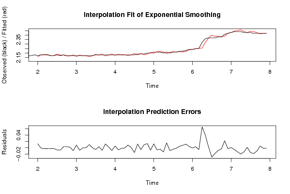
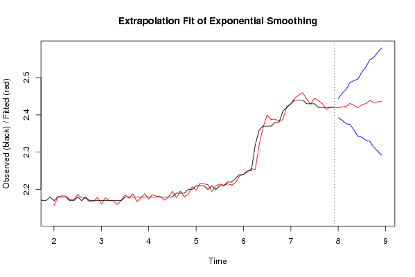
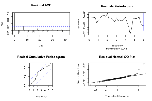
Title produced by software

Exponential Smoothing

Date of computation

Thu, 14 Jan 2010 12:07:55 -0700

Cite this page as follows

Statistical Computations at FreeStatistics.org, Office for Research Development and Education, URL https://freestatistics.org/blog/index.php?v=date/2010/Jan/14/t1263496111w7ezi9tz20sm2zc.htm/, Retrieved Mon, 29 Apr 2024 19:12:54 +0000

Statistical Computations at FreeStatistics.org, Office for Research Development and Education, URL https://freestatistics.org/blog/index.php?pk=72182, Retrieved Mon, 29 Apr 2024 19:12:54 +0000

QR Codes:

Paste this QR Code to cite your computation.

Original text written by user:

IsPrivate?

No (this computation is public)

User-defined keywords

KDGP2W62

Estimated Impact

236

Family? (F = Feedback message, R = changed R code, M = changed R Module, P = changed Parameters, D = changed Data)

-       [Exponential Smoothing] [Gemiddelde consum...] [2010-01-14 19:07:55] [6590c54be3d1f5d26c781440f79f0ebc] [Current]
- R PD    [Exponential Smoothing] [consumptieprijs r...] [2010-01-26 12:42:30] [bf68df4edce3d2e638b253cf289b9d76] 

Feedback Forum

Post a new message

Dataseries X:

Download CSV

Histogram

Boxplots

2,12
2,13
2,14
2,15
2,15
2,16
2,17
2,17
2,18
2,17
2,17
2,18
2,17
2,18
2,18
2,18
2,17
2,17
2,18
2,17
2,18
2,17
2,17
2,17
2,17
2,17
2,17
2,17
2,17
2,17
2,18
2,18
2,18
2,18
2,18
2,18
2,18
2,18
2,18
2,18
2,18
2,18
2,18
2,19
2,19
2,19
2,2
2,2
2,21
2,21
2,21
2,2
2,21
2,2
2,21
2,21
2,22
2,22
2,23
2,24
2,24
2,25
2,25
2,32
2,36
2,37
2,37
2,37
2,38
2,38
2,41
2,42
2,43
2,44
2,44
2,44
2,43
2,43
2,43
2,42
2,42
2,42
2,42
2,42

Summary of computational transaction
Raw Input	view raw input (R code)
Raw Output	view raw output of R engine
Computing time	2 seconds
R Server	'Gwilym Jenkins' @ 72.249.127.135

\begin{tabular}{lllllllll}
\hline
Summary of computational transaction \tabularnewline
Raw Input & view raw input (R code)  \tabularnewline
Raw Output & view raw output of R engine  \tabularnewline
Computing time & 2 seconds \tabularnewline
R Server & 'Gwilym Jenkins' @ 72.249.127.135 \tabularnewline
\hline
\end{tabular}
%Source: https://freestatistics.org/blog/index.php?pk=72182&T=0

[TABLE]
[ROW][C]Summary of computational transaction[/C][/ROW]
[ROW][C]Raw Input[/C][C]view raw input (R code) [/C][/ROW]
[ROW][C]Raw Output[/C][C]view raw output of R engine [/C][/ROW]
[ROW][C]Computing time[/C][C]2 seconds[/C][/ROW]
[ROW][C]R Server[/C][C]'Gwilym Jenkins' @ 72.249.127.135[/C][/ROW]
[/TABLE]
Source: https://freestatistics.org/blog/index.php?pk=72182&T=0

Globally Unique Identifier (entire table): ba.freestatistics.org/blog/index.php?pk=72182&T=0

As an alternative you can also use a QR Code:

The GUIDs for individual cells are displayed in the table below:

Summary of computational transaction
Raw Input	view raw input (R code)
Raw Output	view raw output of R engine
Computing time	2 seconds
R Server	'Gwilym Jenkins' @ 72.249.127.135

Estimated Parameters of Exponential Smoothing
Parameter	Value
alpha	0.88008275007892
beta	0.141425389189999
gamma	1

\begin{tabular}{lllllllll}
\hline
Estimated Parameters of Exponential Smoothing \tabularnewline
Parameter & Value \tabularnewline
alpha & 0.88008275007892 \tabularnewline
beta & 0.141425389189999 \tabularnewline
gamma & 1 \tabularnewline
\hline
\end{tabular}
%Source: https://freestatistics.org/blog/index.php?pk=72182&T=1

[TABLE]
[ROW][C]Estimated Parameters of Exponential Smoothing[/C][/ROW]
[ROW][C]Parameter[/C][C]Value[/C][/ROW]
[ROW][C]alpha[/C][C]0.88008275007892[/C][/ROW]
[ROW][C]beta[/C][C]0.141425389189999[/C][/ROW]
[ROW][C]gamma[/C][C]1[/C][/ROW]
[/TABLE]
Source: https://freestatistics.org/blog/index.php?pk=72182&T=1

Globally Unique Identifier (entire table): ba.freestatistics.org/blog/index.php?pk=72182&T=1

As an alternative you can also use a QR Code:

The GUIDs for individual cells are displayed in the table below:

Estimated Parameters of Exponential Smoothing
Parameter	Value
alpha	0.88008275007892
beta	0.141425389189999
gamma	1

Interpolation Forecasts of Exponential Smoothing
t	Observed	Fitted	Residuals
13	2.17	2.15729700854701	0.0127029914529908
14	2.18	2.18086489286783	-0.000864892867825873
15	2.18	2.18280093311450	-0.00280093311449692
16	2.18	2.18268447666828	-0.00268447666828431
17	2.17	2.17233638533652	-0.00233638533651703
18	2.17	2.17242050920447	-0.00242050920447445
19	2.18	2.18671265923205	-0.006712659232051
20	2.17	2.17722519724388	-0.00722519724387816
21	2.18	2.17680403433087	0.00319596566913338
22	2.17	2.16678547967492	0.00321452032507885
23	2.17	2.16801668661782	0.00198331338218116
24	2.17	2.17924451807540	-0.00924451807539528
25	2.17	2.16138027460692	0.00861972539308375
26	2.17	2.17757724228165	-0.00757724228164536
27	2.17	2.1703879541396	-0.000387954139601021
28	2.17	2.16972367711803	0.000276322881972657
29	2.17	2.15970618867926	0.0102938113207376
30	2.17	2.17015098561080	-0.000150985610804621
31	2.18	2.18546342276160	-0.00546342276159795
32	2.18	2.17670703900138	0.00329296099862342
33	2.18	2.18779466538795	-0.00779466538794837
34	2.18	2.16773997303508	0.0122600269649209
35	2.18	2.17754449191288	0.00245550808712158
36	2.18	2.18866041584772	-0.0086604158477157
37	2.18	2.17434409525091	0.00565590474908717
38	2.18	2.18651309827509	-0.00651309827509117
39	2.18	2.18177765296916	-0.00177765296915622
40	2.18	2.18045220232528	-0.000452202325275319
41	2.18	2.17138636250353	0.00861363749647337
42	2.18	2.17928237293983	0.000717627060168091
43	2.18	2.19501273787818	-0.0150127378781764
44	2.19	2.17800417219209	0.0119958278079140
45	2.19	2.19560661940866	-0.00560661940866325
46	2.19	2.18034000510316	0.009659994896841
47	2.2	2.18681444692766	0.0131855530723439
48	2.2	2.20751013085986	-0.00751013085985663
49	2.21	2.19753552498397	0.0124644750160252
50	2.21	2.21669739064261	-0.00669739064260844
51	2.21	2.21480470700586	-0.00480470700586277
52	2.2	2.21303446989610	-0.0130344698961022
53	2.21	2.19447660609998	0.0155233939000228
54	2.2	2.20886119824393	-0.00886119824392839
55	2.21	2.21443711580331	-0.00443711580331074
56	2.21	2.21145312509673	-0.00145312509673046
57	2.22	2.21491296530842	0.00508703469158345
58	2.22	2.21202380026744	0.00797619973256358
59	2.23	2.21836498128105	0.01163501871895
60	2.24	2.23594715132076	0.0040528486792426
61	2.24	2.24071627656621	-0.00071627656620743
62	2.25	2.24651164835017	0.00348835164982564
63	2.25	2.25560950174062	-0.00560950174061547
64	2.32	2.25384319403829	0.066156805961711
65	2.36	2.31996051741567	0.04003948258433
66	2.37	2.36760431453241	0.00239568546759283
67	2.37	2.39962599631797	-0.0296259963179746
68	2.37	2.38770462924133	-0.0177046292413348
69	2.38	2.38849640942027	-0.00849640942026886
70	2.38	2.38315880313578	-0.00315880313577521
71	2.41	2.38791273882031	0.0220872611796916
72	2.42	2.42285918656155	-0.00285918656154527
73	2.43	2.42918760713903	0.00081239286096757
74	2.44	2.44523716810679	-0.00523716810679264
75	2.44	2.45288344771435	-0.0128834477143540
76	2.44	2.45973471980118	-0.0197347198011837
77	2.43	2.44285113274165	-0.0128511327416478
78	2.43	2.42857224267078	0.00142775732921807
79	2.43	2.44492121302189	-0.0149212130218905
80	2.42	2.43822019328998	-0.0182201932899790
81	2.42	2.43044763228951	-0.0104476322895062
82	2.42	2.41457517193747	0.00542482806253375
83	2.42	2.42152153506199	-0.00152153506199193
84	2.42	2.42137096865162	-0.00137096865162478

\begin{tabular}{lllllllll}
\hline
Interpolation Forecasts of Exponential Smoothing \tabularnewline
t & Observed & Fitted & Residuals \tabularnewline
13 & 2.17 & 2.15729700854701 & 0.0127029914529908 \tabularnewline
14 & 2.18 & 2.18086489286783 & -0.000864892867825873 \tabularnewline
15 & 2.18 & 2.18280093311450 & -0.00280093311449692 \tabularnewline
16 & 2.18 & 2.18268447666828 & -0.00268447666828431 \tabularnewline
17 & 2.17 & 2.17233638533652 & -0.00233638533651703 \tabularnewline
18 & 2.17 & 2.17242050920447 & -0.00242050920447445 \tabularnewline
19 & 2.18 & 2.18671265923205 & -0.006712659232051 \tabularnewline
20 & 2.17 & 2.17722519724388 & -0.00722519724387816 \tabularnewline
21 & 2.18 & 2.17680403433087 & 0.00319596566913338 \tabularnewline
22 & 2.17 & 2.16678547967492 & 0.00321452032507885 \tabularnewline
23 & 2.17 & 2.16801668661782 & 0.00198331338218116 \tabularnewline
24 & 2.17 & 2.17924451807540 & -0.00924451807539528 \tabularnewline
25 & 2.17 & 2.16138027460692 & 0.00861972539308375 \tabularnewline
26 & 2.17 & 2.17757724228165 & -0.00757724228164536 \tabularnewline
27 & 2.17 & 2.1703879541396 & -0.000387954139601021 \tabularnewline
28 & 2.17 & 2.16972367711803 & 0.000276322881972657 \tabularnewline
29 & 2.17 & 2.15970618867926 & 0.0102938113207376 \tabularnewline
30 & 2.17 & 2.17015098561080 & -0.000150985610804621 \tabularnewline
31 & 2.18 & 2.18546342276160 & -0.00546342276159795 \tabularnewline
32 & 2.18 & 2.17670703900138 & 0.00329296099862342 \tabularnewline
33 & 2.18 & 2.18779466538795 & -0.00779466538794837 \tabularnewline
34 & 2.18 & 2.16773997303508 & 0.0122600269649209 \tabularnewline
35 & 2.18 & 2.17754449191288 & 0.00245550808712158 \tabularnewline
36 & 2.18 & 2.18866041584772 & -0.0086604158477157 \tabularnewline
37 & 2.18 & 2.17434409525091 & 0.00565590474908717 \tabularnewline
38 & 2.18 & 2.18651309827509 & -0.00651309827509117 \tabularnewline
39 & 2.18 & 2.18177765296916 & -0.00177765296915622 \tabularnewline
40 & 2.18 & 2.18045220232528 & -0.000452202325275319 \tabularnewline
41 & 2.18 & 2.17138636250353 & 0.00861363749647337 \tabularnewline
42 & 2.18 & 2.17928237293983 & 0.000717627060168091 \tabularnewline
43 & 2.18 & 2.19501273787818 & -0.0150127378781764 \tabularnewline
44 & 2.19 & 2.17800417219209 & 0.0119958278079140 \tabularnewline
45 & 2.19 & 2.19560661940866 & -0.00560661940866325 \tabularnewline
46 & 2.19 & 2.18034000510316 & 0.009659994896841 \tabularnewline
47 & 2.2 & 2.18681444692766 & 0.0131855530723439 \tabularnewline
48 & 2.2 & 2.20751013085986 & -0.00751013085985663 \tabularnewline
49 & 2.21 & 2.19753552498397 & 0.0124644750160252 \tabularnewline
50 & 2.21 & 2.21669739064261 & -0.00669739064260844 \tabularnewline
51 & 2.21 & 2.21480470700586 & -0.00480470700586277 \tabularnewline
52 & 2.2 & 2.21303446989610 & -0.0130344698961022 \tabularnewline
53 & 2.21 & 2.19447660609998 & 0.0155233939000228 \tabularnewline
54 & 2.2 & 2.20886119824393 & -0.00886119824392839 \tabularnewline
55 & 2.21 & 2.21443711580331 & -0.00443711580331074 \tabularnewline
56 & 2.21 & 2.21145312509673 & -0.00145312509673046 \tabularnewline
57 & 2.22 & 2.21491296530842 & 0.00508703469158345 \tabularnewline
58 & 2.22 & 2.21202380026744 & 0.00797619973256358 \tabularnewline
59 & 2.23 & 2.21836498128105 & 0.01163501871895 \tabularnewline
60 & 2.24 & 2.23594715132076 & 0.0040528486792426 \tabularnewline
61 & 2.24 & 2.24071627656621 & -0.00071627656620743 \tabularnewline
62 & 2.25 & 2.24651164835017 & 0.00348835164982564 \tabularnewline
63 & 2.25 & 2.25560950174062 & -0.00560950174061547 \tabularnewline
64 & 2.32 & 2.25384319403829 & 0.066156805961711 \tabularnewline
65 & 2.36 & 2.31996051741567 & 0.04003948258433 \tabularnewline
66 & 2.37 & 2.36760431453241 & 0.00239568546759283 \tabularnewline
67 & 2.37 & 2.39962599631797 & -0.0296259963179746 \tabularnewline
68 & 2.37 & 2.38770462924133 & -0.0177046292413348 \tabularnewline
69 & 2.38 & 2.38849640942027 & -0.00849640942026886 \tabularnewline
70 & 2.38 & 2.38315880313578 & -0.00315880313577521 \tabularnewline
71 & 2.41 & 2.38791273882031 & 0.0220872611796916 \tabularnewline
72 & 2.42 & 2.42285918656155 & -0.00285918656154527 \tabularnewline
73 & 2.43 & 2.42918760713903 & 0.00081239286096757 \tabularnewline
74 & 2.44 & 2.44523716810679 & -0.00523716810679264 \tabularnewline
75 & 2.44 & 2.45288344771435 & -0.0128834477143540 \tabularnewline
76 & 2.44 & 2.45973471980118 & -0.0197347198011837 \tabularnewline
77 & 2.43 & 2.44285113274165 & -0.0128511327416478 \tabularnewline
78 & 2.43 & 2.42857224267078 & 0.00142775732921807 \tabularnewline
79 & 2.43 & 2.44492121302189 & -0.0149212130218905 \tabularnewline
80 & 2.42 & 2.43822019328998 & -0.0182201932899790 \tabularnewline
81 & 2.42 & 2.43044763228951 & -0.0104476322895062 \tabularnewline
82 & 2.42 & 2.41457517193747 & 0.00542482806253375 \tabularnewline
83 & 2.42 & 2.42152153506199 & -0.00152153506199193 \tabularnewline
84 & 2.42 & 2.42137096865162 & -0.00137096865162478 \tabularnewline
\hline
\end{tabular}
%Source: https://freestatistics.org/blog/index.php?pk=72182&T=2

[TABLE]
[ROW][C]Interpolation Forecasts of Exponential Smoothing[/C][/ROW]
[ROW][C]t[/C][C]Observed[/C][C]Fitted[/C][C]Residuals[/C][/ROW]
[ROW][C]13[/C][C]2.17[/C][C]2.15729700854701[/C][C]0.0127029914529908[/C][/ROW]
[ROW][C]14[/C][C]2.18[/C][C]2.18086489286783[/C][C]-0.000864892867825873[/C][/ROW]
[ROW][C]15[/C][C]2.18[/C][C]2.18280093311450[/C][C]-0.00280093311449692[/C][/ROW]
[ROW][C]16[/C][C]2.18[/C][C]2.18268447666828[/C][C]-0.00268447666828431[/C][/ROW]
[ROW][C]17[/C][C]2.17[/C][C]2.17233638533652[/C][C]-0.00233638533651703[/C][/ROW]
[ROW][C]18[/C][C]2.17[/C][C]2.17242050920447[/C][C]-0.00242050920447445[/C][/ROW]
[ROW][C]19[/C][C]2.18[/C][C]2.18671265923205[/C][C]-0.006712659232051[/C][/ROW]
[ROW][C]20[/C][C]2.17[/C][C]2.17722519724388[/C][C]-0.00722519724387816[/C][/ROW]
[ROW][C]21[/C][C]2.18[/C][C]2.17680403433087[/C][C]0.00319596566913338[/C][/ROW]
[ROW][C]22[/C][C]2.17[/C][C]2.16678547967492[/C][C]0.00321452032507885[/C][/ROW]
[ROW][C]23[/C][C]2.17[/C][C]2.16801668661782[/C][C]0.00198331338218116[/C][/ROW]
[ROW][C]24[/C][C]2.17[/C][C]2.17924451807540[/C][C]-0.00924451807539528[/C][/ROW]
[ROW][C]25[/C][C]2.17[/C][C]2.16138027460692[/C][C]0.00861972539308375[/C][/ROW]
[ROW][C]26[/C][C]2.17[/C][C]2.17757724228165[/C][C]-0.00757724228164536[/C][/ROW]
[ROW][C]27[/C][C]2.17[/C][C]2.1703879541396[/C][C]-0.000387954139601021[/C][/ROW]
[ROW][C]28[/C][C]2.17[/C][C]2.16972367711803[/C][C]0.000276322881972657[/C][/ROW]
[ROW][C]29[/C][C]2.17[/C][C]2.15970618867926[/C][C]0.0102938113207376[/C][/ROW]
[ROW][C]30[/C][C]2.17[/C][C]2.17015098561080[/C][C]-0.000150985610804621[/C][/ROW]
[ROW][C]31[/C][C]2.18[/C][C]2.18546342276160[/C][C]-0.00546342276159795[/C][/ROW]
[ROW][C]32[/C][C]2.18[/C][C]2.17670703900138[/C][C]0.00329296099862342[/C][/ROW]
[ROW][C]33[/C][C]2.18[/C][C]2.18779466538795[/C][C]-0.00779466538794837[/C][/ROW]
[ROW][C]34[/C][C]2.18[/C][C]2.16773997303508[/C][C]0.0122600269649209[/C][/ROW]
[ROW][C]35[/C][C]2.18[/C][C]2.17754449191288[/C][C]0.00245550808712158[/C][/ROW]
[ROW][C]36[/C][C]2.18[/C][C]2.18866041584772[/C][C]-0.0086604158477157[/C][/ROW]
[ROW][C]37[/C][C]2.18[/C][C]2.17434409525091[/C][C]0.00565590474908717[/C][/ROW]
[ROW][C]38[/C][C]2.18[/C][C]2.18651309827509[/C][C]-0.00651309827509117[/C][/ROW]
[ROW][C]39[/C][C]2.18[/C][C]2.18177765296916[/C][C]-0.00177765296915622[/C][/ROW]
[ROW][C]40[/C][C]2.18[/C][C]2.18045220232528[/C][C]-0.000452202325275319[/C][/ROW]
[ROW][C]41[/C][C]2.18[/C][C]2.17138636250353[/C][C]0.00861363749647337[/C][/ROW]
[ROW][C]42[/C][C]2.18[/C][C]2.17928237293983[/C][C]0.000717627060168091[/C][/ROW]
[ROW][C]43[/C][C]2.18[/C][C]2.19501273787818[/C][C]-0.0150127378781764[/C][/ROW]
[ROW][C]44[/C][C]2.19[/C][C]2.17800417219209[/C][C]0.0119958278079140[/C][/ROW]
[ROW][C]45[/C][C]2.19[/C][C]2.19560661940866[/C][C]-0.00560661940866325[/C][/ROW]
[ROW][C]46[/C][C]2.19[/C][C]2.18034000510316[/C][C]0.009659994896841[/C][/ROW]
[ROW][C]47[/C][C]2.2[/C][C]2.18681444692766[/C][C]0.0131855530723439[/C][/ROW]
[ROW][C]48[/C][C]2.2[/C][C]2.20751013085986[/C][C]-0.00751013085985663[/C][/ROW]
[ROW][C]49[/C][C]2.21[/C][C]2.19753552498397[/C][C]0.0124644750160252[/C][/ROW]
[ROW][C]50[/C][C]2.21[/C][C]2.21669739064261[/C][C]-0.00669739064260844[/C][/ROW]
[ROW][C]51[/C][C]2.21[/C][C]2.21480470700586[/C][C]-0.00480470700586277[/C][/ROW]
[ROW][C]52[/C][C]2.2[/C][C]2.21303446989610[/C][C]-0.0130344698961022[/C][/ROW]
[ROW][C]53[/C][C]2.21[/C][C]2.19447660609998[/C][C]0.0155233939000228[/C][/ROW]
[ROW][C]54[/C][C]2.2[/C][C]2.20886119824393[/C][C]-0.00886119824392839[/C][/ROW]
[ROW][C]55[/C][C]2.21[/C][C]2.21443711580331[/C][C]-0.00443711580331074[/C][/ROW]
[ROW][C]56[/C][C]2.21[/C][C]2.21145312509673[/C][C]-0.00145312509673046[/C][/ROW]
[ROW][C]57[/C][C]2.22[/C][C]2.21491296530842[/C][C]0.00508703469158345[/C][/ROW]
[ROW][C]58[/C][C]2.22[/C][C]2.21202380026744[/C][C]0.00797619973256358[/C][/ROW]
[ROW][C]59[/C][C]2.23[/C][C]2.21836498128105[/C][C]0.01163501871895[/C][/ROW]
[ROW][C]60[/C][C]2.24[/C][C]2.23594715132076[/C][C]0.0040528486792426[/C][/ROW]
[ROW][C]61[/C][C]2.24[/C][C]2.24071627656621[/C][C]-0.00071627656620743[/C][/ROW]
[ROW][C]62[/C][C]2.25[/C][C]2.24651164835017[/C][C]0.00348835164982564[/C][/ROW]
[ROW][C]63[/C][C]2.25[/C][C]2.25560950174062[/C][C]-0.00560950174061547[/C][/ROW]
[ROW][C]64[/C][C]2.32[/C][C]2.25384319403829[/C][C]0.066156805961711[/C][/ROW]
[ROW][C]65[/C][C]2.36[/C][C]2.31996051741567[/C][C]0.04003948258433[/C][/ROW]
[ROW][C]66[/C][C]2.37[/C][C]2.36760431453241[/C][C]0.00239568546759283[/C][/ROW]
[ROW][C]67[/C][C]2.37[/C][C]2.39962599631797[/C][C]-0.0296259963179746[/C][/ROW]
[ROW][C]68[/C][C]2.37[/C][C]2.38770462924133[/C][C]-0.0177046292413348[/C][/ROW]
[ROW][C]69[/C][C]2.38[/C][C]2.38849640942027[/C][C]-0.00849640942026886[/C][/ROW]
[ROW][C]70[/C][C]2.38[/C][C]2.38315880313578[/C][C]-0.00315880313577521[/C][/ROW]
[ROW][C]71[/C][C]2.41[/C][C]2.38791273882031[/C][C]0.0220872611796916[/C][/ROW]
[ROW][C]72[/C][C]2.42[/C][C]2.42285918656155[/C][C]-0.00285918656154527[/C][/ROW]
[ROW][C]73[/C][C]2.43[/C][C]2.42918760713903[/C][C]0.00081239286096757[/C][/ROW]
[ROW][C]74[/C][C]2.44[/C][C]2.44523716810679[/C][C]-0.00523716810679264[/C][/ROW]
[ROW][C]75[/C][C]2.44[/C][C]2.45288344771435[/C][C]-0.0128834477143540[/C][/ROW]
[ROW][C]76[/C][C]2.44[/C][C]2.45973471980118[/C][C]-0.0197347198011837[/C][/ROW]
[ROW][C]77[/C][C]2.43[/C][C]2.44285113274165[/C][C]-0.0128511327416478[/C][/ROW]
[ROW][C]78[/C][C]2.43[/C][C]2.42857224267078[/C][C]0.00142775732921807[/C][/ROW]
[ROW][C]79[/C][C]2.43[/C][C]2.44492121302189[/C][C]-0.0149212130218905[/C][/ROW]
[ROW][C]80[/C][C]2.42[/C][C]2.43822019328998[/C][C]-0.0182201932899790[/C][/ROW]
[ROW][C]81[/C][C]2.42[/C][C]2.43044763228951[/C][C]-0.0104476322895062[/C][/ROW]
[ROW][C]82[/C][C]2.42[/C][C]2.41457517193747[/C][C]0.00542482806253375[/C][/ROW]
[ROW][C]83[/C][C]2.42[/C][C]2.42152153506199[/C][C]-0.00152153506199193[/C][/ROW]
[ROW][C]84[/C][C]2.42[/C][C]2.42137096865162[/C][C]-0.00137096865162478[/C][/ROW]
[/TABLE]
Source: https://freestatistics.org/blog/index.php?pk=72182&T=2

Globally Unique Identifier (entire table): ba.freestatistics.org/blog/index.php?pk=72182&T=2

As an alternative you can also use a QR Code:

The GUIDs for individual cells are displayed in the table below:

Interpolation Forecasts of Exponential Smoothing
t	Observed	Fitted	Residuals
13	2.17	2.15729700854701	0.0127029914529908
14	2.18	2.18086489286783	-0.000864892867825873
15	2.18	2.18280093311450	-0.00280093311449692
16	2.18	2.18268447666828	-0.00268447666828431
17	2.17	2.17233638533652	-0.00233638533651703
18	2.17	2.17242050920447	-0.00242050920447445
19	2.18	2.18671265923205	-0.006712659232051
20	2.17	2.17722519724388	-0.00722519724387816
21	2.18	2.17680403433087	0.00319596566913338
22	2.17	2.16678547967492	0.00321452032507885
23	2.17	2.16801668661782	0.00198331338218116
24	2.17	2.17924451807540	-0.00924451807539528
25	2.17	2.16138027460692	0.00861972539308375
26	2.17	2.17757724228165	-0.00757724228164536
27	2.17	2.1703879541396	-0.000387954139601021
28	2.17	2.16972367711803	0.000276322881972657
29	2.17	2.15970618867926	0.0102938113207376
30	2.17	2.17015098561080	-0.000150985610804621
31	2.18	2.18546342276160	-0.00546342276159795
32	2.18	2.17670703900138	0.00329296099862342
33	2.18	2.18779466538795	-0.00779466538794837
34	2.18	2.16773997303508	0.0122600269649209
35	2.18	2.17754449191288	0.00245550808712158
36	2.18	2.18866041584772	-0.0086604158477157
37	2.18	2.17434409525091	0.00565590474908717
38	2.18	2.18651309827509	-0.00651309827509117
39	2.18	2.18177765296916	-0.00177765296915622
40	2.18	2.18045220232528	-0.000452202325275319
41	2.18	2.17138636250353	0.00861363749647337
42	2.18	2.17928237293983	0.000717627060168091
43	2.18	2.19501273787818	-0.0150127378781764
44	2.19	2.17800417219209	0.0119958278079140
45	2.19	2.19560661940866	-0.00560661940866325
46	2.19	2.18034000510316	0.009659994896841
47	2.2	2.18681444692766	0.0131855530723439
48	2.2	2.20751013085986	-0.00751013085985663
49	2.21	2.19753552498397	0.0124644750160252
50	2.21	2.21669739064261	-0.00669739064260844
51	2.21	2.21480470700586	-0.00480470700586277
52	2.2	2.21303446989610	-0.0130344698961022
53	2.21	2.19447660609998	0.0155233939000228
54	2.2	2.20886119824393	-0.00886119824392839
55	2.21	2.21443711580331	-0.00443711580331074
56	2.21	2.21145312509673	-0.00145312509673046
57	2.22	2.21491296530842	0.00508703469158345
58	2.22	2.21202380026744	0.00797619973256358
59	2.23	2.21836498128105	0.01163501871895
60	2.24	2.23594715132076	0.0040528486792426
61	2.24	2.24071627656621	-0.00071627656620743
62	2.25	2.24651164835017	0.00348835164982564
63	2.25	2.25560950174062	-0.00560950174061547
64	2.32	2.25384319403829	0.066156805961711
65	2.36	2.31996051741567	0.04003948258433
66	2.37	2.36760431453241	0.00239568546759283
67	2.37	2.39962599631797	-0.0296259963179746
68	2.37	2.38770462924133	-0.0177046292413348
69	2.38	2.38849640942027	-0.00849640942026886
70	2.38	2.38315880313578	-0.00315880313577521
71	2.41	2.38791273882031	0.0220872611796916
72	2.42	2.42285918656155	-0.00285918656154527
73	2.43	2.42918760713903	0.00081239286096757
74	2.44	2.44523716810679	-0.00523716810679264
75	2.44	2.45288344771435	-0.0128834477143540
76	2.44	2.45973471980118	-0.0197347198011837
77	2.43	2.44285113274165	-0.0128511327416478
78	2.43	2.42857224267078	0.00142775732921807
79	2.43	2.44492121302189	-0.0149212130218905
80	2.42	2.43822019328998	-0.0182201932899790
81	2.42	2.43044763228951	-0.0104476322895062
82	2.42	2.41457517193747	0.00542482806253375
83	2.42	2.42152153506199	-0.00152153506199193
84	2.42	2.42137096865162	-0.00137096865162478

Extrapolation Forecasts of Exponential Smoothing
t	Forecast	95% Lower Bound	95% Upper Bound
85	2.41830685202448	2.3927560780378	2.44385762601116
86	2.42167230018505	2.38545577217708	2.45788882819302
87	2.42241895673412	2.37611779018755	2.46872012328069
88	2.43079885145166	2.37450006983472	2.48709763306861
89	2.42557692247115	2.35917565247378	2.49197819246852
90	2.41938791832089	2.34268881172194	2.49608702491984
91	2.42740965364956	2.34017059650561	2.51464871079351
92	2.43019194898317	2.33214575341954	2.5282381445468
93	2.43840154286245	2.32926772379222	2.54753536193269
94	2.43394243365998	2.3134340004082	2.55445086691176
95	2.43492149192300	2.30274902914536	2.56709395470063
96	2.43595741873769	2.29183160511311	2.58008323236226

\begin{tabular}{lllllllll}
\hline
Extrapolation Forecasts of Exponential Smoothing \tabularnewline
t & Forecast & 95% Lower Bound & 95% Upper Bound \tabularnewline
85 & 2.41830685202448 & 2.3927560780378 & 2.44385762601116 \tabularnewline
86 & 2.42167230018505 & 2.38545577217708 & 2.45788882819302 \tabularnewline
87 & 2.42241895673412 & 2.37611779018755 & 2.46872012328069 \tabularnewline
88 & 2.43079885145166 & 2.37450006983472 & 2.48709763306861 \tabularnewline
89 & 2.42557692247115 & 2.35917565247378 & 2.49197819246852 \tabularnewline
90 & 2.41938791832089 & 2.34268881172194 & 2.49608702491984 \tabularnewline
91 & 2.42740965364956 & 2.34017059650561 & 2.51464871079351 \tabularnewline
92 & 2.43019194898317 & 2.33214575341954 & 2.5282381445468 \tabularnewline
93 & 2.43840154286245 & 2.32926772379222 & 2.54753536193269 \tabularnewline
94 & 2.43394243365998 & 2.3134340004082 & 2.55445086691176 \tabularnewline
95 & 2.43492149192300 & 2.30274902914536 & 2.56709395470063 \tabularnewline
96 & 2.43595741873769 & 2.29183160511311 & 2.58008323236226 \tabularnewline
\hline
\end{tabular}
%Source: https://freestatistics.org/blog/index.php?pk=72182&T=3

[TABLE]
[ROW][C]Extrapolation Forecasts of Exponential Smoothing[/C][/ROW]
[ROW][C]t[/C][C]Forecast[/C][C]95% Lower Bound[/C][C]95% Upper Bound[/C][/ROW]
[ROW][C]85[/C][C]2.41830685202448[/C][C]2.3927560780378[/C][C]2.44385762601116[/C][/ROW]
[ROW][C]86[/C][C]2.42167230018505[/C][C]2.38545577217708[/C][C]2.45788882819302[/C][/ROW]
[ROW][C]87[/C][C]2.42241895673412[/C][C]2.37611779018755[/C][C]2.46872012328069[/C][/ROW]
[ROW][C]88[/C][C]2.43079885145166[/C][C]2.37450006983472[/C][C]2.48709763306861[/C][/ROW]
[ROW][C]89[/C][C]2.42557692247115[/C][C]2.35917565247378[/C][C]2.49197819246852[/C][/ROW]
[ROW][C]90[/C][C]2.41938791832089[/C][C]2.34268881172194[/C][C]2.49608702491984[/C][/ROW]
[ROW][C]91[/C][C]2.42740965364956[/C][C]2.34017059650561[/C][C]2.51464871079351[/C][/ROW]
[ROW][C]92[/C][C]2.43019194898317[/C][C]2.33214575341954[/C][C]2.5282381445468[/C][/ROW]
[ROW][C]93[/C][C]2.43840154286245[/C][C]2.32926772379222[/C][C]2.54753536193269[/C][/ROW]
[ROW][C]94[/C][C]2.43394243365998[/C][C]2.3134340004082[/C][C]2.55445086691176[/C][/ROW]
[ROW][C]95[/C][C]2.43492149192300[/C][C]2.30274902914536[/C][C]2.56709395470063[/C][/ROW]
[ROW][C]96[/C][C]2.43595741873769[/C][C]2.29183160511311[/C][C]2.58008323236226[/C][/ROW]
[/TABLE]
Source: https://freestatistics.org/blog/index.php?pk=72182&T=3

Globally Unique Identifier (entire table): ba.freestatistics.org/blog/index.php?pk=72182&T=3

As an alternative you can also use a QR Code:

The GUIDs for individual cells are displayed in the table below:

Extrapolation Forecasts of Exponential Smoothing
t	Forecast	95% Lower Bound	95% Upper Bound
85	2.41830685202448	2.3927560780378	2.44385762601116
86	2.42167230018505	2.38545577217708	2.45788882819302
87	2.42241895673412	2.37611779018755	2.46872012328069
88	2.43079885145166	2.37450006983472	2.48709763306861
89	2.42557692247115	2.35917565247378	2.49197819246852
90	2.41938791832089	2.34268881172194	2.49608702491984
91	2.42740965364956	2.34017059650561	2.51464871079351
92	2.43019194898317	2.33214575341954	2.5282381445468
93	2.43840154286245	2.32926772379222	2.54753536193269
94	2.43394243365998	2.3134340004082	2.55445086691176
95	2.43492149192300	2.30274902914536	2.56709395470063
96	2.43595741873769	2.29183160511311	2.58008323236226

Figure 1

PNG link

Postscript link

PDF link

Figure 2

PNG link

Postscript link

PDF link

Figure 3

PNG link

Postscript link

PDF link

Parameters (Session):

par1 = 12 ; par2 = Triple ; par3 = additive ;

Parameters (R input):

par1 = 12 ; par2 = Triple ; par3 = additive ;

R code (references can be found in the software module):

par1 <- as.numeric(par1)
if (par2 == 'Single') K <- 1
if (par2 == 'Double') K <- 2
if (par2 == 'Triple') K <- par1
nx <- length(x)
nxmK <- nx - K
x <- ts(x, frequency = par1)
if (par2 == 'Single') fit <- HoltWinters(x, gamma=0, beta=0)
if (par2 == 'Double') fit <- HoltWinters(x, gamma=0)
if (par2 == 'Triple') fit <- HoltWinters(x, seasonal=par3)
fit
myresid <- x - fit$fitted[,'xhat']
bitmap(file='test1.png')
op <- par(mfrow=c(2,1))
plot(fit,ylab='Observed (black) / Fitted (red)',main='Interpolation Fit of Exponential Smoothing')
plot(myresid,ylab='Residuals',main='Interpolation Prediction Errors')
par(op)
dev.off()
bitmap(file='test2.png')
p <- predict(fit, par1, prediction.interval=TRUE)
np <- length(p[,1])
plot(fit,p,ylab='Observed (black) / Fitted (red)',main='Extrapolation Fit of Exponential Smoothing')
dev.off()
bitmap(file='test3.png')
op <- par(mfrow = c(2,2))
acf(as.numeric(myresid),lag.max = nx/2,main='Residual ACF')
spectrum(myresid,main='Residals Periodogram')
cpgram(myresid,main='Residal Cumulative Periodogram')
qqnorm(myresid,main='Residual Normal QQ Plot')
qqline(myresid)
par(op)
dev.off()
load(file='createtable')
a<-table.start()
a<-table.row.start(a)
a<-table.element(a,'Estimated Parameters of Exponential Smoothing',2,TRUE)
a<-table.row.end(a)
a<-table.row.start(a)
a<-table.element(a,'Parameter',header=TRUE)
a<-table.element(a,'Value',header=TRUE)
a<-table.row.end(a)
a<-table.row.start(a)
a<-table.element(a,'alpha',header=TRUE)
a<-table.element(a,fit$alpha)
a<-table.row.end(a)
a<-table.row.start(a)
a<-table.element(a,'beta',header=TRUE)
a<-table.element(a,fit$beta)
a<-table.row.end(a)
a<-table.row.start(a)
a<-table.element(a,'gamma',header=TRUE)
a<-table.element(a,fit$gamma)
a<-table.row.end(a)
a<-table.end(a)
table.save(a,file='mytable.tab')
a<-table.start()
a<-table.row.start(a)
a<-table.element(a,'Interpolation Forecasts of Exponential Smoothing',4,TRUE)
a<-table.row.end(a)
a<-table.row.start(a)
a<-table.element(a,'t',header=TRUE)
a<-table.element(a,'Observed',header=TRUE)
a<-table.element(a,'Fitted',header=TRUE)
a<-table.element(a,'Residuals',header=TRUE)
a<-table.row.end(a)
for (i in 1:nxmK) {
a<-table.row.start(a)
a<-table.element(a,i+K,header=TRUE)
a<-table.element(a,x[i+K])
a<-table.element(a,fit$fitted[i,'xhat'])
a<-table.element(a,myresid[i])
a<-table.row.end(a)
}
a<-table.end(a)
table.save(a,file='mytable1.tab')
a<-table.start()
a<-table.row.start(a)
a<-table.element(a,'Extrapolation Forecasts of Exponential Smoothing',4,TRUE)
a<-table.row.end(a)
a<-table.row.start(a)
a<-table.element(a,'t',header=TRUE)
a<-table.element(a,'Forecast',header=TRUE)
a<-table.element(a,'95% Lower Bound',header=TRUE)
a<-table.element(a,'95% Upper Bound',header=TRUE)
a<-table.row.end(a)
for (i in 1:np) {
a<-table.row.start(a)
a<-table.element(a,nx+i,header=TRUE)
a<-table.element(a,p[i,'fit'])
a<-table.element(a,p[i,'lwr'])
a<-table.element(a,p[i,'upr'])
a<-table.row.end(a)
}
a<-table.end(a)
table.save(a,file='mytable2.tab')

Free Statistics

Description of Statistical Computation

Tree of Dependent Computations

Dataset

Tables (Output of Computation)

Figures (Output of Computation)

Input Parameters & R Code