Repository of Reproducible Computations

Free Statistics

of Irreproducible Research!

Author's title

Author

*The author of this computation has been verified*

R Software Module

rwasp_autocorrelation.wasp

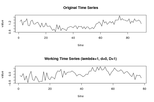
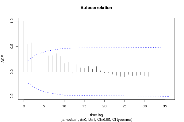
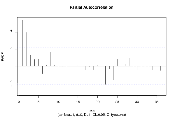
Title produced by software

(Partial) Autocorrelation Function

Date of computation

Wed, 29 Dec 2010 13:04:46 +0000

Cite this page as follows

Statistical Computations at FreeStatistics.org, Office for Research Development and Education, URL https://freestatistics.org/blog/index.php?v=date/2010/Dec/29/t1293627752xagwuxncl4ag5pn.htm/, Retrieved Fri, 03 May 2024 06:01:32 +0000

Statistical Computations at FreeStatistics.org, Office for Research Development and Education, URL https://freestatistics.org/blog/index.php?pk=116781, Retrieved Fri, 03 May 2024 06:01:32 +0000

QR Codes:

Paste this QR Code to cite your computation.

Original text written by user:

IsPrivate?

No (this computation is public)

User-defined keywords

Estimated Impact

181

Family? (F = Feedback message, R = changed R code, M = changed R Module, P = changed Parameters, D = changed Data)

-     [Univariate Explorative Data Analysis] [Run Sequence gebo...] [2008-12-12 13:32:37] [76963dc1903f0f612b6153510a3818cf]
- R  D  [Univariate Explorative Data Analysis] [Run Sequence gebo...] [2008-12-17 12:14:40] [76963dc1903f0f612b6153510a3818cf]
-         [Univariate Explorative Data Analysis] [Run Sequence Plot...] [2008-12-22 18:19:51] [1ce0d16c8f4225c977b42c8fa93bc163]
- RMP       [(Partial) Autocorrelation Function] [Identifying Integ...] [2009-11-22 12:16:10] [b98453cac15ba1066b407e146608df68]
-    D        [(Partial) Autocorrelation Function] [] [2009-11-24 09:55:25] [fef2f8976fa1eef1b54e2cee317fe737]
-    D          [(Partial) Autocorrelation Function] [] [2009-12-18 11:14:21] [fef2f8976fa1eef1b54e2cee317fe737]
- R               [(Partial) Autocorrelation Function] [Paper: ACF] [2010-12-22 20:09:28] [29e492448d11757ae0fad5ef6e7f8e86]
-   PD                [(Partial) Autocorrelation Function] [] [2010-12-29 13:04:46] [e180d4cd19004beeddc12e67012247dc] [Current]

Feedback Forum

Post a new message

Dataseries X:

Download CSV

Histogram

Boxplots

Summary of computational transaction
Raw Input	view raw input (R code)
Raw Output	view raw output of R engine
Computing time	2 seconds
R Server	'Gwilym Jenkins' @ 72.249.127.135

\begin{tabular}{lllllllll}
\hline
Summary of computational transaction \tabularnewline
Raw Input & view raw input (R code)  \tabularnewline
Raw Output & view raw output of R engine  \tabularnewline
Computing time & 2 seconds \tabularnewline
R Server & 'Gwilym Jenkins' @ 72.249.127.135 \tabularnewline
\hline
\end{tabular}
%Source: https://freestatistics.org/blog/index.php?pk=116781&T=0

[TABLE]
[ROW][C]Summary of computational transaction[/C][/ROW]
[ROW][C]Raw Input[/C][C]view raw input (R code) [/C][/ROW]
[ROW][C]Raw Output[/C][C]view raw output of R engine [/C][/ROW]
[ROW][C]Computing time[/C][C]2 seconds[/C][/ROW]
[ROW][C]R Server[/C][C]'Gwilym Jenkins' @ 72.249.127.135[/C][/ROW]
[/TABLE]
Source: https://freestatistics.org/blog/index.php?pk=116781&T=0

Globally Unique Identifier (entire table): ba.freestatistics.org/blog/index.php?pk=116781&T=0

As an alternative you can also use a QR Code:

The GUIDs for individual cells are displayed in the table below:

Summary of computational transaction
Raw Input	view raw input (R code)
Raw Output	view raw output of R engine
Computing time	2 seconds
R Server	'Gwilym Jenkins' @ 72.249.127.135

Autocorrelation Function
Time lag k	ACF(k)	T-STAT	P-value
1	0.540793	4.7762	4e-06
2	0.573057	5.0611	1e-06
3	0.477042	4.2131	3.4e-05
4	0.449183	3.9671	8e-05
5	0.42536	3.7567	0.000165
6	0.316004	2.7909	0.003303
7	0.321021	2.8352	0.002915
8	0.358574	3.1668	0.0011
9	0.304344	2.6879	0.004393
10	0.164735	1.4549	0.074854
11	0.189818	1.6764	0.048829
12	-0.028712	-0.2536	0.400244
13	0.141743	1.2518	0.107185
14	0.079485	0.702	0.242388
15	0.066233	0.585	0.280133
16	0.106719	0.9425	0.174419
17	0.055775	0.4926	0.311842
18	0.104471	0.9227	0.179514
19	0.020125	0.1777	0.429695
20	-0.022	-0.1943	0.423222
21	-0.013719	-0.1212	0.451937
22	-0.048421	-0.4276	0.335044
23	-0.071695	-0.6332	0.264231
24	-0.090752	-0.8015	0.212638
25	-0.102974	-0.9094	0.182958
26	-0.052378	-0.4626	0.322473
27	-0.077695	-0.6862	0.247317
28	-0.071909	-0.6351	0.263615
29	-0.068659	-0.6064	0.273011
30	-0.084151	-0.7432	0.229795
31	-0.090565	-0.7998	0.213114
32	-0.137618	-1.2154	0.113939
33	-0.179732	-1.5874	0.058239
34	-0.095989	-0.8477	0.199586
35	-0.127458	-1.1257	0.131876
36	-0.113096	-0.9988	0.160481

\begin{tabular}{lllllllll}
\hline
Autocorrelation Function \tabularnewline
Time lag k & ACF(k) & T-STAT & P-value \tabularnewline
1 & 0.540793 & 4.7762 & 4e-06 \tabularnewline
2 & 0.573057 & 5.0611 & 1e-06 \tabularnewline
3 & 0.477042 & 4.2131 & 3.4e-05 \tabularnewline
4 & 0.449183 & 3.9671 & 8e-05 \tabularnewline
5 & 0.42536 & 3.7567 & 0.000165 \tabularnewline
6 & 0.316004 & 2.7909 & 0.003303 \tabularnewline
7 & 0.321021 & 2.8352 & 0.002915 \tabularnewline
8 & 0.358574 & 3.1668 & 0.0011 \tabularnewline
9 & 0.304344 & 2.6879 & 0.004393 \tabularnewline
10 & 0.164735 & 1.4549 & 0.074854 \tabularnewline
11 & 0.189818 & 1.6764 & 0.048829 \tabularnewline
12 & -0.028712 & -0.2536 & 0.400244 \tabularnewline
13 & 0.141743 & 1.2518 & 0.107185 \tabularnewline
14 & 0.079485 & 0.702 & 0.242388 \tabularnewline
15 & 0.066233 & 0.585 & 0.280133 \tabularnewline
16 & 0.106719 & 0.9425 & 0.174419 \tabularnewline
17 & 0.055775 & 0.4926 & 0.311842 \tabularnewline
18 & 0.104471 & 0.9227 & 0.179514 \tabularnewline
19 & 0.020125 & 0.1777 & 0.429695 \tabularnewline
20 & -0.022 & -0.1943 & 0.423222 \tabularnewline
21 & -0.013719 & -0.1212 & 0.451937 \tabularnewline
22 & -0.048421 & -0.4276 & 0.335044 \tabularnewline
23 & -0.071695 & -0.6332 & 0.264231 \tabularnewline
24 & -0.090752 & -0.8015 & 0.212638 \tabularnewline
25 & -0.102974 & -0.9094 & 0.182958 \tabularnewline
26 & -0.052378 & -0.4626 & 0.322473 \tabularnewline
27 & -0.077695 & -0.6862 & 0.247317 \tabularnewline
28 & -0.071909 & -0.6351 & 0.263615 \tabularnewline
29 & -0.068659 & -0.6064 & 0.273011 \tabularnewline
30 & -0.084151 & -0.7432 & 0.229795 \tabularnewline
31 & -0.090565 & -0.7998 & 0.213114 \tabularnewline
32 & -0.137618 & -1.2154 & 0.113939 \tabularnewline
33 & -0.179732 & -1.5874 & 0.058239 \tabularnewline
34 & -0.095989 & -0.8477 & 0.199586 \tabularnewline
35 & -0.127458 & -1.1257 & 0.131876 \tabularnewline
36 & -0.113096 & -0.9988 & 0.160481 \tabularnewline
\hline
\end{tabular}
%Source: https://freestatistics.org/blog/index.php?pk=116781&T=1

[TABLE]
[ROW][C]Autocorrelation Function[/C][/ROW]
[ROW][C]Time lag k[/C][C]ACF(k)[/C][C]T-STAT[/C][C]P-value[/C][/ROW]
[ROW][C]1[/C][C]0.540793[/C][C]4.7762[/C][C]4e-06[/C][/ROW]
[ROW][C]2[/C][C]0.573057[/C][C]5.0611[/C][C]1e-06[/C][/ROW]
[ROW][C]3[/C][C]0.477042[/C][C]4.2131[/C][C]3.4e-05[/C][/ROW]
[ROW][C]4[/C][C]0.449183[/C][C]3.9671[/C][C]8e-05[/C][/ROW]
[ROW][C]5[/C][C]0.42536[/C][C]3.7567[/C][C]0.000165[/C][/ROW]
[ROW][C]6[/C][C]0.316004[/C][C]2.7909[/C][C]0.003303[/C][/ROW]
[ROW][C]7[/C][C]0.321021[/C][C]2.8352[/C][C]0.002915[/C][/ROW]
[ROW][C]8[/C][C]0.358574[/C][C]3.1668[/C][C]0.0011[/C][/ROW]
[ROW][C]9[/C][C]0.304344[/C][C]2.6879[/C][C]0.004393[/C][/ROW]
[ROW][C]10[/C][C]0.164735[/C][C]1.4549[/C][C]0.074854[/C][/ROW]
[ROW][C]11[/C][C]0.189818[/C][C]1.6764[/C][C]0.048829[/C][/ROW]
[ROW][C]12[/C][C]-0.028712[/C][C]-0.2536[/C][C]0.400244[/C][/ROW]
[ROW][C]13[/C][C]0.141743[/C][C]1.2518[/C][C]0.107185[/C][/ROW]
[ROW][C]14[/C][C]0.079485[/C][C]0.702[/C][C]0.242388[/C][/ROW]
[ROW][C]15[/C][C]0.066233[/C][C]0.585[/C][C]0.280133[/C][/ROW]
[ROW][C]16[/C][C]0.106719[/C][C]0.9425[/C][C]0.174419[/C][/ROW]
[ROW][C]17[/C][C]0.055775[/C][C]0.4926[/C][C]0.311842[/C][/ROW]
[ROW][C]18[/C][C]0.104471[/C][C]0.9227[/C][C]0.179514[/C][/ROW]
[ROW][C]19[/C][C]0.020125[/C][C]0.1777[/C][C]0.429695[/C][/ROW]
[ROW][C]20[/C][C]-0.022[/C][C]-0.1943[/C][C]0.423222[/C][/ROW]
[ROW][C]21[/C][C]-0.013719[/C][C]-0.1212[/C][C]0.451937[/C][/ROW]
[ROW][C]22[/C][C]-0.048421[/C][C]-0.4276[/C][C]0.335044[/C][/ROW]
[ROW][C]23[/C][C]-0.071695[/C][C]-0.6332[/C][C]0.264231[/C][/ROW]
[ROW][C]24[/C][C]-0.090752[/C][C]-0.8015[/C][C]0.212638[/C][/ROW]
[ROW][C]25[/C][C]-0.102974[/C][C]-0.9094[/C][C]0.182958[/C][/ROW]
[ROW][C]26[/C][C]-0.052378[/C][C]-0.4626[/C][C]0.322473[/C][/ROW]
[ROW][C]27[/C][C]-0.077695[/C][C]-0.6862[/C][C]0.247317[/C][/ROW]
[ROW][C]28[/C][C]-0.071909[/C][C]-0.6351[/C][C]0.263615[/C][/ROW]
[ROW][C]29[/C][C]-0.068659[/C][C]-0.6064[/C][C]0.273011[/C][/ROW]
[ROW][C]30[/C][C]-0.084151[/C][C]-0.7432[/C][C]0.229795[/C][/ROW]
[ROW][C]31[/C][C]-0.090565[/C][C]-0.7998[/C][C]0.213114[/C][/ROW]
[ROW][C]32[/C][C]-0.137618[/C][C]-1.2154[/C][C]0.113939[/C][/ROW]
[ROW][C]33[/C][C]-0.179732[/C][C]-1.5874[/C][C]0.058239[/C][/ROW]
[ROW][C]34[/C][C]-0.095989[/C][C]-0.8477[/C][C]0.199586[/C][/ROW]
[ROW][C]35[/C][C]-0.127458[/C][C]-1.1257[/C][C]0.131876[/C][/ROW]
[ROW][C]36[/C][C]-0.113096[/C][C]-0.9988[/C][C]0.160481[/C][/ROW]
[/TABLE]
Source: https://freestatistics.org/blog/index.php?pk=116781&T=1

Globally Unique Identifier (entire table): ba.freestatistics.org/blog/index.php?pk=116781&T=1

As an alternative you can also use a QR Code:

The GUIDs for individual cells are displayed in the table below:

Autocorrelation Function
Time lag k	ACF(k)	T-STAT	P-value
1	0.540793	4.7762	4e-06
2	0.573057	5.0611	1e-06
3	0.477042	4.2131	3.4e-05
4	0.449183	3.9671	8e-05
5	0.42536	3.7567	0.000165
6	0.316004	2.7909	0.003303
7	0.321021	2.8352	0.002915
8	0.358574	3.1668	0.0011
9	0.304344	2.6879	0.004393
10	0.164735	1.4549	0.074854
11	0.189818	1.6764	0.048829
12	-0.028712	-0.2536	0.400244
13	0.141743	1.2518	0.107185
14	0.079485	0.702	0.242388
15	0.066233	0.585	0.280133
16	0.106719	0.9425	0.174419
17	0.055775	0.4926	0.311842
18	0.104471	0.9227	0.179514
19	0.020125	0.1777	0.429695
20	-0.022	-0.1943	0.423222
21	-0.013719	-0.1212	0.451937
22	-0.048421	-0.4276	0.335044
23	-0.071695	-0.6332	0.264231
24	-0.090752	-0.8015	0.212638
25	-0.102974	-0.9094	0.182958
26	-0.052378	-0.4626	0.322473
27	-0.077695	-0.6862	0.247317
28	-0.071909	-0.6351	0.263615
29	-0.068659	-0.6064	0.273011
30	-0.084151	-0.7432	0.229795
31	-0.090565	-0.7998	0.213114
32	-0.137618	-1.2154	0.113939
33	-0.179732	-1.5874	0.058239
34	-0.095989	-0.8477	0.199586
35	-0.127458	-1.1257	0.131876
36	-0.113096	-0.9988	0.160481

Partial Autocorrelation Function
Time lag k	PACF(k)	T-STAT	P-value
1	0.540793	4.7762	4e-06
2	0.396584	3.5025	0.000383
3	0.12674	1.1193	0.133215
4	0.07736	0.6832	0.248245
5	0.080914	0.7146	0.238489
6	-0.088618	-0.7827	0.218099
7	0.01457	0.1287	0.448972
8	0.16534	1.4602	0.07412
9	0.015115	0.1335	0.447075
10	-0.240961	-2.1281	0.018243
11	-0.003232	-0.0285	0.48865
12	-0.313084	-2.7651	0.00355
13	0.186447	1.6467	0.051826
14	0.191005	1.6869	0.047808
15	0.00485	0.0428	0.482973
16	0.0291	0.257	0.398926
17	-0.042542	-0.3757	0.354071
18	-0.006043	-0.0534	0.478787
19	-0.042245	-0.3731	0.355043
20	0.00374	0.033	0.486868
21	0.002457	0.0217	0.491371
22	-0.216311	-1.9104	0.029878
23	-0.035695	-0.3152	0.376707
24	-0.163209	-1.4414	0.076734
25	0.078299	0.6915	0.245646
26	0.23311	2.0588	0.021427
27	0.024898	0.2199	0.413263
28	0.091432	0.8075	0.210915
29	-0.067799	-0.5988	0.275526
30	-0.043982	-0.3884	0.349376
31	-0.059818	-0.5283	0.299396
32	-0.125876	-1.1117	0.13484
33	-0.102633	-0.9064	0.18375
34	-0.04572	-0.4038	0.343737
35	-0.001349	-0.0119	0.495261
36	-0.052292	-0.4618	0.322745

\begin{tabular}{lllllllll}
\hline
Partial Autocorrelation Function \tabularnewline
Time lag k & PACF(k) & T-STAT & P-value \tabularnewline
1 & 0.540793 & 4.7762 & 4e-06 \tabularnewline
2 & 0.396584 & 3.5025 & 0.000383 \tabularnewline
3 & 0.12674 & 1.1193 & 0.133215 \tabularnewline
4 & 0.07736 & 0.6832 & 0.248245 \tabularnewline
5 & 0.080914 & 0.7146 & 0.238489 \tabularnewline
6 & -0.088618 & -0.7827 & 0.218099 \tabularnewline
7 & 0.01457 & 0.1287 & 0.448972 \tabularnewline
8 & 0.16534 & 1.4602 & 0.07412 \tabularnewline
9 & 0.015115 & 0.1335 & 0.447075 \tabularnewline
10 & -0.240961 & -2.1281 & 0.018243 \tabularnewline
11 & -0.003232 & -0.0285 & 0.48865 \tabularnewline
12 & -0.313084 & -2.7651 & 0.00355 \tabularnewline
13 & 0.186447 & 1.6467 & 0.051826 \tabularnewline
14 & 0.191005 & 1.6869 & 0.047808 \tabularnewline
15 & 0.00485 & 0.0428 & 0.482973 \tabularnewline
16 & 0.0291 & 0.257 & 0.398926 \tabularnewline
17 & -0.042542 & -0.3757 & 0.354071 \tabularnewline
18 & -0.006043 & -0.0534 & 0.478787 \tabularnewline
19 & -0.042245 & -0.3731 & 0.355043 \tabularnewline
20 & 0.00374 & 0.033 & 0.486868 \tabularnewline
21 & 0.002457 & 0.0217 & 0.491371 \tabularnewline
22 & -0.216311 & -1.9104 & 0.029878 \tabularnewline
23 & -0.035695 & -0.3152 & 0.376707 \tabularnewline
24 & -0.163209 & -1.4414 & 0.076734 \tabularnewline
25 & 0.078299 & 0.6915 & 0.245646 \tabularnewline
26 & 0.23311 & 2.0588 & 0.021427 \tabularnewline
27 & 0.024898 & 0.2199 & 0.413263 \tabularnewline
28 & 0.091432 & 0.8075 & 0.210915 \tabularnewline
29 & -0.067799 & -0.5988 & 0.275526 \tabularnewline
30 & -0.043982 & -0.3884 & 0.349376 \tabularnewline
31 & -0.059818 & -0.5283 & 0.299396 \tabularnewline
32 & -0.125876 & -1.1117 & 0.13484 \tabularnewline
33 & -0.102633 & -0.9064 & 0.18375 \tabularnewline
34 & -0.04572 & -0.4038 & 0.343737 \tabularnewline
35 & -0.001349 & -0.0119 & 0.495261 \tabularnewline
36 & -0.052292 & -0.4618 & 0.322745 \tabularnewline
\hline
\end{tabular}
%Source: https://freestatistics.org/blog/index.php?pk=116781&T=2

[TABLE]
[ROW][C]Partial Autocorrelation Function[/C][/ROW]
[ROW][C]Time lag k[/C][C]PACF(k)[/C][C]T-STAT[/C][C]P-value[/C][/ROW]
[ROW][C]1[/C][C]0.540793[/C][C]4.7762[/C][C]4e-06[/C][/ROW]
[ROW][C]2[/C][C]0.396584[/C][C]3.5025[/C][C]0.000383[/C][/ROW]
[ROW][C]3[/C][C]0.12674[/C][C]1.1193[/C][C]0.133215[/C][/ROW]
[ROW][C]4[/C][C]0.07736[/C][C]0.6832[/C][C]0.248245[/C][/ROW]
[ROW][C]5[/C][C]0.080914[/C][C]0.7146[/C][C]0.238489[/C][/ROW]
[ROW][C]6[/C][C]-0.088618[/C][C]-0.7827[/C][C]0.218099[/C][/ROW]
[ROW][C]7[/C][C]0.01457[/C][C]0.1287[/C][C]0.448972[/C][/ROW]
[ROW][C]8[/C][C]0.16534[/C][C]1.4602[/C][C]0.07412[/C][/ROW]
[ROW][C]9[/C][C]0.015115[/C][C]0.1335[/C][C]0.447075[/C][/ROW]
[ROW][C]10[/C][C]-0.240961[/C][C]-2.1281[/C][C]0.018243[/C][/ROW]
[ROW][C]11[/C][C]-0.003232[/C][C]-0.0285[/C][C]0.48865[/C][/ROW]
[ROW][C]12[/C][C]-0.313084[/C][C]-2.7651[/C][C]0.00355[/C][/ROW]
[ROW][C]13[/C][C]0.186447[/C][C]1.6467[/C][C]0.051826[/C][/ROW]
[ROW][C]14[/C][C]0.191005[/C][C]1.6869[/C][C]0.047808[/C][/ROW]
[ROW][C]15[/C][C]0.00485[/C][C]0.0428[/C][C]0.482973[/C][/ROW]
[ROW][C]16[/C][C]0.0291[/C][C]0.257[/C][C]0.398926[/C][/ROW]
[ROW][C]17[/C][C]-0.042542[/C][C]-0.3757[/C][C]0.354071[/C][/ROW]
[ROW][C]18[/C][C]-0.006043[/C][C]-0.0534[/C][C]0.478787[/C][/ROW]
[ROW][C]19[/C][C]-0.042245[/C][C]-0.3731[/C][C]0.355043[/C][/ROW]
[ROW][C]20[/C][C]0.00374[/C][C]0.033[/C][C]0.486868[/C][/ROW]
[ROW][C]21[/C][C]0.002457[/C][C]0.0217[/C][C]0.491371[/C][/ROW]
[ROW][C]22[/C][C]-0.216311[/C][C]-1.9104[/C][C]0.029878[/C][/ROW]
[ROW][C]23[/C][C]-0.035695[/C][C]-0.3152[/C][C]0.376707[/C][/ROW]
[ROW][C]24[/C][C]-0.163209[/C][C]-1.4414[/C][C]0.076734[/C][/ROW]
[ROW][C]25[/C][C]0.078299[/C][C]0.6915[/C][C]0.245646[/C][/ROW]
[ROW][C]26[/C][C]0.23311[/C][C]2.0588[/C][C]0.021427[/C][/ROW]
[ROW][C]27[/C][C]0.024898[/C][C]0.2199[/C][C]0.413263[/C][/ROW]
[ROW][C]28[/C][C]0.091432[/C][C]0.8075[/C][C]0.210915[/C][/ROW]
[ROW][C]29[/C][C]-0.067799[/C][C]-0.5988[/C][C]0.275526[/C][/ROW]
[ROW][C]30[/C][C]-0.043982[/C][C]-0.3884[/C][C]0.349376[/C][/ROW]
[ROW][C]31[/C][C]-0.059818[/C][C]-0.5283[/C][C]0.299396[/C][/ROW]
[ROW][C]32[/C][C]-0.125876[/C][C]-1.1117[/C][C]0.13484[/C][/ROW]
[ROW][C]33[/C][C]-0.102633[/C][C]-0.9064[/C][C]0.18375[/C][/ROW]
[ROW][C]34[/C][C]-0.04572[/C][C]-0.4038[/C][C]0.343737[/C][/ROW]
[ROW][C]35[/C][C]-0.001349[/C][C]-0.0119[/C][C]0.495261[/C][/ROW]
[ROW][C]36[/C][C]-0.052292[/C][C]-0.4618[/C][C]0.322745[/C][/ROW]
[/TABLE]
Source: https://freestatistics.org/blog/index.php?pk=116781&T=2

Globally Unique Identifier (entire table): ba.freestatistics.org/blog/index.php?pk=116781&T=2

As an alternative you can also use a QR Code:

The GUIDs for individual cells are displayed in the table below:

Partial Autocorrelation Function
Time lag k	PACF(k)	T-STAT	P-value
1	0.540793	4.7762	4e-06
2	0.396584	3.5025	0.000383
3	0.12674	1.1193	0.133215
4	0.07736	0.6832	0.248245
5	0.080914	0.7146	0.238489
6	-0.088618	-0.7827	0.218099
7	0.01457	0.1287	0.448972
8	0.16534	1.4602	0.07412
9	0.015115	0.1335	0.447075
10	-0.240961	-2.1281	0.018243
11	-0.003232	-0.0285	0.48865
12	-0.313084	-2.7651	0.00355
13	0.186447	1.6467	0.051826
14	0.191005	1.6869	0.047808
15	0.00485	0.0428	0.482973
16	0.0291	0.257	0.398926
17	-0.042542	-0.3757	0.354071
18	-0.006043	-0.0534	0.478787
19	-0.042245	-0.3731	0.355043
20	0.00374	0.033	0.486868
21	0.002457	0.0217	0.491371
22	-0.216311	-1.9104	0.029878
23	-0.035695	-0.3152	0.376707
24	-0.163209	-1.4414	0.076734
25	0.078299	0.6915	0.245646
26	0.23311	2.0588	0.021427
27	0.024898	0.2199	0.413263
28	0.091432	0.8075	0.210915
29	-0.067799	-0.5988	0.275526
30	-0.043982	-0.3884	0.349376
31	-0.059818	-0.5283	0.299396
32	-0.125876	-1.1117	0.13484
33	-0.102633	-0.9064	0.18375
34	-0.04572	-0.4038	0.343737
35	-0.001349	-0.0119	0.495261
36	-0.052292	-0.4618	0.322745

Figure 1

PNG link

Postscript link

PDF link

Figure 2

PNG link

Postscript link

PDF link

Figure 3

PNG link

Postscript link

PDF link

Parameters (Session):

par1 = 36 ; par2 = 1 ; par3 = 0 ; par4 = 1 ; par5 = 12 ; par6 = MA ; par7 = 0.95 ;

Parameters (R input):

par1 = 36 ; par2 = 1 ; par3 = 0 ; par4 = 1 ; par5 = 12 ; par6 = MA ; par7 = 0.95 ; par8 = ;

R code (references can be found in the software module):

if (par1 == 'Default') {
par1 = 10*log10(length(x))
} else {
par1 <- as.numeric(par1)
}
par2 <- as.numeric(par2)
par3 <- as.numeric(par3)
par4 <- as.numeric(par4)
par5 <- as.numeric(par5)
if (par6 == 'White Noise') par6 <- 'white' else par6 <- 'ma'
par7 <- as.numeric(par7)
if (par8 != '') par8 <- as.numeric(par8)
ox <- x
if (par8 == '') {
if (par2 == 0) {
x <- log(x)
} else {
x <- (x ^ par2 - 1) / par2
}
} else {
x <- log(x,base=par8)
}
if (par3 > 0) x <- diff(x,lag=1,difference=par3)
if (par4 > 0) x <- diff(x,lag=par5,difference=par4)
bitmap(file='picts.png')
op <- par(mfrow=c(2,1))
plot(ox,type='l',main='Original Time Series',xlab='time',ylab='value')
if (par8=='') {
mytitle <- paste('Working Time Series (lambda=',par2,', d=',par3,', D=',par4,')',sep='')
mysub <- paste('(lambda=',par2,', d=',par3,', D=',par4,', CI=', par7, ', CI type=',par6,')',sep='')
} else {
mytitle <- paste('Working Time Series (base=',par8,', d=',par3,', D=',par4,')',sep='')
mysub <- paste('(base=',par8,', d=',par3,', D=',par4,', CI=', par7, ', CI type=',par6,')',sep='')
}
plot(x,type='l', main=mytitle,xlab='time',ylab='value')
par(op)
dev.off()
bitmap(file='pic1.png')
racf <- acf(x, par1, main='Autocorrelation', xlab='time lag', ylab='ACF', ci.type=par6, ci=par7, sub=mysub)
dev.off()
bitmap(file='pic2.png')
rpacf <- pacf(x,par1,main='Partial Autocorrelation',xlab='lags',ylab='PACF',sub=mysub)
dev.off()
(myacf <- c(racf$acf))
(mypacf <- c(rpacf$acf))
lengthx <- length(x)
sqrtn <- sqrt(lengthx)
load(file='createtable')
a<-table.start()
a<-table.row.start(a)
a<-table.element(a,'Autocorrelation Function',4,TRUE)
a<-table.row.end(a)
a<-table.row.start(a)
a<-table.element(a,'Time lag k',header=TRUE)
a<-table.element(a,hyperlink('basics.htm','ACF(k)','click here for more information about the Autocorrelation Function'),header=TRUE)
a<-table.element(a,'T-STAT',header=TRUE)
a<-table.element(a,'P-value',header=TRUE)
a<-table.row.end(a)
for (i in 2:(par1+1)) {
a<-table.row.start(a)
a<-table.element(a,i-1,header=TRUE)
a<-table.element(a,round(myacf[i],6))
mytstat <- myacf[i]*sqrtn
a<-table.element(a,round(mytstat,4))
a<-table.element(a,round(1-pt(abs(mytstat),lengthx),6))
a<-table.row.end(a)
}
a<-table.end(a)
table.save(a,file='mytable.tab')
a<-table.start()
a<-table.row.start(a)
a<-table.element(a,'Partial Autocorrelation Function',4,TRUE)
a<-table.row.end(a)
a<-table.row.start(a)
a<-table.element(a,'Time lag k',header=TRUE)
a<-table.element(a,hyperlink('basics.htm','PACF(k)','click here for more information about the Partial Autocorrelation Function'),header=TRUE)
a<-table.element(a,'T-STAT',header=TRUE)
a<-table.element(a,'P-value',header=TRUE)
a<-table.row.end(a)
for (i in 1:par1) {
a<-table.row.start(a)
a<-table.element(a,i,header=TRUE)
a<-table.element(a,round(mypacf[i],6))
mytstat <- mypacf[i]*sqrtn
a<-table.element(a,round(mytstat,4))
a<-table.element(a,round(1-pt(abs(mytstat),lengthx),6))
a<-table.row.end(a)
}
a<-table.end(a)
table.save(a,file='mytable1.tab')

Free Statistics

Description of Statistical Computation

Tree of Dependent Computations

Dataset

Tables (Output of Computation)

Figures (Output of Computation)

Input Parameters & R Code