Repository of Reproducible Computations

Free Statistics

of Irreproducible Research!

Author's title

Author

*The author of this computation has been verified*

R Software Module

rwasp_autocorrelation.wasp

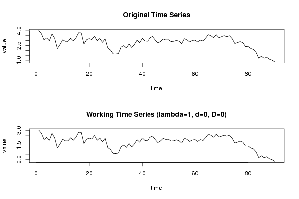
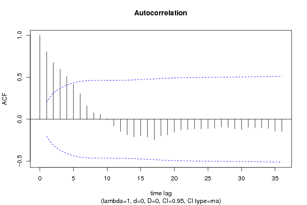
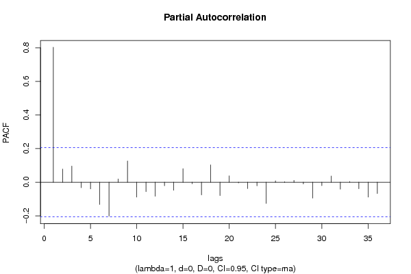
Title produced by software

(Partial) Autocorrelation Function

Date of computation

Wed, 29 Dec 2010 12:46:43 +0000

Cite this page as follows

Statistical Computations at FreeStatistics.org, Office for Research Development and Education, URL https://freestatistics.org/blog/index.php?v=date/2010/Dec/29/t1293626671r0xhbp7hkfaiugr.htm/, Retrieved Fri, 03 May 2024 11:24:38 +0000

Statistical Computations at FreeStatistics.org, Office for Research Development and Education, URL https://freestatistics.org/blog/index.php?pk=116766, Retrieved Fri, 03 May 2024 11:24:38 +0000

QR Codes:

Paste this QR Code to cite your computation.

Original text written by user:

IsPrivate?

No (this computation is public)

User-defined keywords

Estimated Impact

150

Family? (F = Feedback message, R = changed R code, M = changed R Module, P = changed Parameters, D = changed Data)

-     [Univariate Explorative Data Analysis] [Run Sequence gebo...] [2008-12-12 13:32:37] [76963dc1903f0f612b6153510a3818cf]
- R  D  [Univariate Explorative Data Analysis] [Run Sequence gebo...] [2008-12-17 12:14:40] [76963dc1903f0f612b6153510a3818cf]
-         [Univariate Explorative Data Analysis] [Run Sequence Plot...] [2008-12-22 18:19:51] [1ce0d16c8f4225c977b42c8fa93bc163]
- RMP       [(Partial) Autocorrelation Function] [Identifying Integ...] [2009-11-22 12:16:10] [b98453cac15ba1066b407e146608df68]
-    D        [(Partial) Autocorrelation Function] [] [2009-11-24 09:55:25] [fef2f8976fa1eef1b54e2cee317fe737]
-    D          [(Partial) Autocorrelation Function] [] [2009-12-18 11:14:21] [fef2f8976fa1eef1b54e2cee317fe737]
- R               [(Partial) Autocorrelation Function] [Paper: ACF] [2010-12-22 20:09:28] [29e492448d11757ae0fad5ef6e7f8e86]
-    D                [(Partial) Autocorrelation Function] [] [2010-12-29 12:46:43] [e180d4cd19004beeddc12e67012247dc] [Current]

Feedback Forum

Post a new message

Dataseries X:

Download CSV

Histogram

Boxplots

Summary of computational transaction
Raw Input	view raw input (R code)
Raw Output	view raw output of R engine
Computing time	2 seconds
R Server	'RServer@AstonUniversity' @ vre.aston.ac.uk

\begin{tabular}{lllllllll}
\hline
Summary of computational transaction \tabularnewline
Raw Input & view raw input (R code)  \tabularnewline
Raw Output & view raw output of R engine  \tabularnewline
Computing time & 2 seconds \tabularnewline
R Server & 'RServer@AstonUniversity' @ vre.aston.ac.uk \tabularnewline
\hline
\end{tabular}
%Source: https://freestatistics.org/blog/index.php?pk=116766&T=0

[TABLE]
[ROW][C]Summary of computational transaction[/C][/ROW]
[ROW][C]Raw Input[/C][C]view raw input (R code) [/C][/ROW]
[ROW][C]Raw Output[/C][C]view raw output of R engine [/C][/ROW]
[ROW][C]Computing time[/C][C]2 seconds[/C][/ROW]
[ROW][C]R Server[/C][C]'RServer@AstonUniversity' @ vre.aston.ac.uk[/C][/ROW]
[/TABLE]
Source: https://freestatistics.org/blog/index.php?pk=116766&T=0

Globally Unique Identifier (entire table): ba.freestatistics.org/blog/index.php?pk=116766&T=0

As an alternative you can also use a QR Code:

The GUIDs for individual cells are displayed in the table below:

Summary of computational transaction
Raw Input	view raw input (R code)
Raw Output	view raw output of R engine
Computing time	2 seconds
R Server	'RServer@AstonUniversity' @ vre.aston.ac.uk

Autocorrelation Function
Time lag k	ACF(k)	T-STAT	P-value
1	0.803941	7.6269	0
2	0.673983	6.394	0
3	0.596061	5.6547	0
4	0.507816	4.8176	3e-06
5	0.419103	3.976	7.1e-05
6	0.305589	2.8991	0.002351
7	0.159552	1.5136	0.06681
8	0.079312	0.7524	0.22688
9	0.061104	0.5797	0.281787
10	-0.009155	-0.0869	0.465492
11	-0.080281	-0.7616	0.22414
12	-0.146893	-1.3936	0.083442
13	-0.187019	-1.7742	0.039704
14	-0.209324	-1.9858	0.025048
15	-0.195477	-1.8545	0.033474
16	-0.211873	-2.01	0.023713
17	-0.242828	-2.3037	0.011772
18	-0.198215	-1.8804	0.031641
19	-0.185892	-1.7635	0.040603
20	-0.15534	-1.4737	0.072028
21	-0.126551	-1.2006	0.116535
22	-0.123806	-1.1745	0.121642
23	-0.115599	-1.0967	0.137856
24	-0.115221	-1.0931	0.138638
25	-0.110949	-1.0526	0.147681
26	-0.106458	-1.01	0.157612
27	-0.093563	-0.8876	0.188556
28	-0.09721	-0.9222	0.179442
29	-0.115193	-1.0928	0.138696
30	-0.120702	-1.1451	0.127606
31	-0.095556	-0.9065	0.183539
32	-0.101542	-0.9633	0.168987
33	-0.103835	-0.9851	0.163616
34	-0.110362	-1.047	0.148955
35	-0.142992	-1.3565	0.08916
36	-0.145837	-1.3835	0.084961

\begin{tabular}{lllllllll}
\hline
Autocorrelation Function \tabularnewline
Time lag k & ACF(k) & T-STAT & P-value \tabularnewline
1 & 0.803941 & 7.6269 & 0 \tabularnewline
2 & 0.673983 & 6.394 & 0 \tabularnewline
3 & 0.596061 & 5.6547 & 0 \tabularnewline
4 & 0.507816 & 4.8176 & 3e-06 \tabularnewline
5 & 0.419103 & 3.976 & 7.1e-05 \tabularnewline
6 & 0.305589 & 2.8991 & 0.002351 \tabularnewline
7 & 0.159552 & 1.5136 & 0.06681 \tabularnewline
8 & 0.079312 & 0.7524 & 0.22688 \tabularnewline
9 & 0.061104 & 0.5797 & 0.281787 \tabularnewline
10 & -0.009155 & -0.0869 & 0.465492 \tabularnewline
11 & -0.080281 & -0.7616 & 0.22414 \tabularnewline
12 & -0.146893 & -1.3936 & 0.083442 \tabularnewline
13 & -0.187019 & -1.7742 & 0.039704 \tabularnewline
14 & -0.209324 & -1.9858 & 0.025048 \tabularnewline
15 & -0.195477 & -1.8545 & 0.033474 \tabularnewline
16 & -0.211873 & -2.01 & 0.023713 \tabularnewline
17 & -0.242828 & -2.3037 & 0.011772 \tabularnewline
18 & -0.198215 & -1.8804 & 0.031641 \tabularnewline
19 & -0.185892 & -1.7635 & 0.040603 \tabularnewline
20 & -0.15534 & -1.4737 & 0.072028 \tabularnewline
21 & -0.126551 & -1.2006 & 0.116535 \tabularnewline
22 & -0.123806 & -1.1745 & 0.121642 \tabularnewline
23 & -0.115599 & -1.0967 & 0.137856 \tabularnewline
24 & -0.115221 & -1.0931 & 0.138638 \tabularnewline
25 & -0.110949 & -1.0526 & 0.147681 \tabularnewline
26 & -0.106458 & -1.01 & 0.157612 \tabularnewline
27 & -0.093563 & -0.8876 & 0.188556 \tabularnewline
28 & -0.09721 & -0.9222 & 0.179442 \tabularnewline
29 & -0.115193 & -1.0928 & 0.138696 \tabularnewline
30 & -0.120702 & -1.1451 & 0.127606 \tabularnewline
31 & -0.095556 & -0.9065 & 0.183539 \tabularnewline
32 & -0.101542 & -0.9633 & 0.168987 \tabularnewline
33 & -0.103835 & -0.9851 & 0.163616 \tabularnewline
34 & -0.110362 & -1.047 & 0.148955 \tabularnewline
35 & -0.142992 & -1.3565 & 0.08916 \tabularnewline
36 & -0.145837 & -1.3835 & 0.084961 \tabularnewline
\hline
\end{tabular}
%Source: https://freestatistics.org/blog/index.php?pk=116766&T=1

[TABLE]
[ROW][C]Autocorrelation Function[/C][/ROW]
[ROW][C]Time lag k[/C][C]ACF(k)[/C][C]T-STAT[/C][C]P-value[/C][/ROW]
[ROW][C]1[/C][C]0.803941[/C][C]7.6269[/C][C]0[/C][/ROW]
[ROW][C]2[/C][C]0.673983[/C][C]6.394[/C][C]0[/C][/ROW]
[ROW][C]3[/C][C]0.596061[/C][C]5.6547[/C][C]0[/C][/ROW]
[ROW][C]4[/C][C]0.507816[/C][C]4.8176[/C][C]3e-06[/C][/ROW]
[ROW][C]5[/C][C]0.419103[/C][C]3.976[/C][C]7.1e-05[/C][/ROW]
[ROW][C]6[/C][C]0.305589[/C][C]2.8991[/C][C]0.002351[/C][/ROW]
[ROW][C]7[/C][C]0.159552[/C][C]1.5136[/C][C]0.06681[/C][/ROW]
[ROW][C]8[/C][C]0.079312[/C][C]0.7524[/C][C]0.22688[/C][/ROW]
[ROW][C]9[/C][C]0.061104[/C][C]0.5797[/C][C]0.281787[/C][/ROW]
[ROW][C]10[/C][C]-0.009155[/C][C]-0.0869[/C][C]0.465492[/C][/ROW]
[ROW][C]11[/C][C]-0.080281[/C][C]-0.7616[/C][C]0.22414[/C][/ROW]
[ROW][C]12[/C][C]-0.146893[/C][C]-1.3936[/C][C]0.083442[/C][/ROW]
[ROW][C]13[/C][C]-0.187019[/C][C]-1.7742[/C][C]0.039704[/C][/ROW]
[ROW][C]14[/C][C]-0.209324[/C][C]-1.9858[/C][C]0.025048[/C][/ROW]
[ROW][C]15[/C][C]-0.195477[/C][C]-1.8545[/C][C]0.033474[/C][/ROW]
[ROW][C]16[/C][C]-0.211873[/C][C]-2.01[/C][C]0.023713[/C][/ROW]
[ROW][C]17[/C][C]-0.242828[/C][C]-2.3037[/C][C]0.011772[/C][/ROW]
[ROW][C]18[/C][C]-0.198215[/C][C]-1.8804[/C][C]0.031641[/C][/ROW]
[ROW][C]19[/C][C]-0.185892[/C][C]-1.7635[/C][C]0.040603[/C][/ROW]
[ROW][C]20[/C][C]-0.15534[/C][C]-1.4737[/C][C]0.072028[/C][/ROW]
[ROW][C]21[/C][C]-0.126551[/C][C]-1.2006[/C][C]0.116535[/C][/ROW]
[ROW][C]22[/C][C]-0.123806[/C][C]-1.1745[/C][C]0.121642[/C][/ROW]
[ROW][C]23[/C][C]-0.115599[/C][C]-1.0967[/C][C]0.137856[/C][/ROW]
[ROW][C]24[/C][C]-0.115221[/C][C]-1.0931[/C][C]0.138638[/C][/ROW]
[ROW][C]25[/C][C]-0.110949[/C][C]-1.0526[/C][C]0.147681[/C][/ROW]
[ROW][C]26[/C][C]-0.106458[/C][C]-1.01[/C][C]0.157612[/C][/ROW]
[ROW][C]27[/C][C]-0.093563[/C][C]-0.8876[/C][C]0.188556[/C][/ROW]
[ROW][C]28[/C][C]-0.09721[/C][C]-0.9222[/C][C]0.179442[/C][/ROW]
[ROW][C]29[/C][C]-0.115193[/C][C]-1.0928[/C][C]0.138696[/C][/ROW]
[ROW][C]30[/C][C]-0.120702[/C][C]-1.1451[/C][C]0.127606[/C][/ROW]
[ROW][C]31[/C][C]-0.095556[/C][C]-0.9065[/C][C]0.183539[/C][/ROW]
[ROW][C]32[/C][C]-0.101542[/C][C]-0.9633[/C][C]0.168987[/C][/ROW]
[ROW][C]33[/C][C]-0.103835[/C][C]-0.9851[/C][C]0.163616[/C][/ROW]
[ROW][C]34[/C][C]-0.110362[/C][C]-1.047[/C][C]0.148955[/C][/ROW]
[ROW][C]35[/C][C]-0.142992[/C][C]-1.3565[/C][C]0.08916[/C][/ROW]
[ROW][C]36[/C][C]-0.145837[/C][C]-1.3835[/C][C]0.084961[/C][/ROW]
[/TABLE]
Source: https://freestatistics.org/blog/index.php?pk=116766&T=1

Globally Unique Identifier (entire table): ba.freestatistics.org/blog/index.php?pk=116766&T=1

As an alternative you can also use a QR Code:

The GUIDs for individual cells are displayed in the table below:

Autocorrelation Function
Time lag k	ACF(k)	T-STAT	P-value
1	0.803941	7.6269	0
2	0.673983	6.394	0
3	0.596061	5.6547	0
4	0.507816	4.8176	3e-06
5	0.419103	3.976	7.1e-05
6	0.305589	2.8991	0.002351
7	0.159552	1.5136	0.06681
8	0.079312	0.7524	0.22688
9	0.061104	0.5797	0.281787
10	-0.009155	-0.0869	0.465492
11	-0.080281	-0.7616	0.22414
12	-0.146893	-1.3936	0.083442
13	-0.187019	-1.7742	0.039704
14	-0.209324	-1.9858	0.025048
15	-0.195477	-1.8545	0.033474
16	-0.211873	-2.01	0.023713
17	-0.242828	-2.3037	0.011772
18	-0.198215	-1.8804	0.031641
19	-0.185892	-1.7635	0.040603
20	-0.15534	-1.4737	0.072028
21	-0.126551	-1.2006	0.116535
22	-0.123806	-1.1745	0.121642
23	-0.115599	-1.0967	0.137856
24	-0.115221	-1.0931	0.138638
25	-0.110949	-1.0526	0.147681
26	-0.106458	-1.01	0.157612
27	-0.093563	-0.8876	0.188556
28	-0.09721	-0.9222	0.179442
29	-0.115193	-1.0928	0.138696
30	-0.120702	-1.1451	0.127606
31	-0.095556	-0.9065	0.183539
32	-0.101542	-0.9633	0.168987
33	-0.103835	-0.9851	0.163616
34	-0.110362	-1.047	0.148955
35	-0.142992	-1.3565	0.08916
36	-0.145837	-1.3835	0.084961

Partial Autocorrelation Function
Time lag k	PACF(k)	T-STAT	P-value
1	0.803941	7.6269	0
2	0.078212	0.742	0.230014
3	0.095926	0.91	0.182618
4	-0.032595	-0.3092	0.378932
5	-0.040088	-0.3803	0.352305
6	-0.132718	-1.2591	0.10563
7	-0.201543	-1.912	0.029528
8	0.019804	0.1879	0.4257
9	0.126713	1.2021	0.116239
10	-0.088991	-0.8442	0.200387
11	-0.056046	-0.5317	0.298122
12	-0.083936	-0.7963	0.21398
13	-0.020985	-0.1991	0.421325
14	-0.048119	-0.4565	0.324567
15	0.080979	0.7682	0.222181
16	-0.009022	-0.0856	0.465992
17	-0.075853	-0.7196	0.236817
18	0.102996	0.9771	0.165569
19	-0.079762	-0.7567	0.225605
20	0.037968	0.3602	0.359774
21	-0.004422	-0.042	0.483314
22	-0.037517	-0.3559	0.361367
23	-0.021715	-0.206	0.418624
24	-0.126912	-1.204	0.115874
25	0.008575	0.0813	0.467674
26	0.003169	0.0301	0.488043
27	0.01078	0.1023	0.459385
28	-0.009935	-0.0943	0.462559
29	-0.094537	-0.8969	0.186093
30	-0.020186	-0.1915	0.424281
31	0.036861	0.3497	0.363694
32	-0.041275	-0.3916	0.348151
33	0.004358	0.0413	0.483558
34	-0.03904	-0.3704	0.35599
35	-0.088443	-0.839	0.201835
36	-0.067487	-0.6402	0.261823

\begin{tabular}{lllllllll}
\hline
Partial Autocorrelation Function \tabularnewline
Time lag k & PACF(k) & T-STAT & P-value \tabularnewline
1 & 0.803941 & 7.6269 & 0 \tabularnewline
2 & 0.078212 & 0.742 & 0.230014 \tabularnewline
3 & 0.095926 & 0.91 & 0.182618 \tabularnewline
4 & -0.032595 & -0.3092 & 0.378932 \tabularnewline
5 & -0.040088 & -0.3803 & 0.352305 \tabularnewline
6 & -0.132718 & -1.2591 & 0.10563 \tabularnewline
7 & -0.201543 & -1.912 & 0.029528 \tabularnewline
8 & 0.019804 & 0.1879 & 0.4257 \tabularnewline
9 & 0.126713 & 1.2021 & 0.116239 \tabularnewline
10 & -0.088991 & -0.8442 & 0.200387 \tabularnewline
11 & -0.056046 & -0.5317 & 0.298122 \tabularnewline
12 & -0.083936 & -0.7963 & 0.21398 \tabularnewline
13 & -0.020985 & -0.1991 & 0.421325 \tabularnewline
14 & -0.048119 & -0.4565 & 0.324567 \tabularnewline
15 & 0.080979 & 0.7682 & 0.222181 \tabularnewline
16 & -0.009022 & -0.0856 & 0.465992 \tabularnewline
17 & -0.075853 & -0.7196 & 0.236817 \tabularnewline
18 & 0.102996 & 0.9771 & 0.165569 \tabularnewline
19 & -0.079762 & -0.7567 & 0.225605 \tabularnewline
20 & 0.037968 & 0.3602 & 0.359774 \tabularnewline
21 & -0.004422 & -0.042 & 0.483314 \tabularnewline
22 & -0.037517 & -0.3559 & 0.361367 \tabularnewline
23 & -0.021715 & -0.206 & 0.418624 \tabularnewline
24 & -0.126912 & -1.204 & 0.115874 \tabularnewline
25 & 0.008575 & 0.0813 & 0.467674 \tabularnewline
26 & 0.003169 & 0.0301 & 0.488043 \tabularnewline
27 & 0.01078 & 0.1023 & 0.459385 \tabularnewline
28 & -0.009935 & -0.0943 & 0.462559 \tabularnewline
29 & -0.094537 & -0.8969 & 0.186093 \tabularnewline
30 & -0.020186 & -0.1915 & 0.424281 \tabularnewline
31 & 0.036861 & 0.3497 & 0.363694 \tabularnewline
32 & -0.041275 & -0.3916 & 0.348151 \tabularnewline
33 & 0.004358 & 0.0413 & 0.483558 \tabularnewline
34 & -0.03904 & -0.3704 & 0.35599 \tabularnewline
35 & -0.088443 & -0.839 & 0.201835 \tabularnewline
36 & -0.067487 & -0.6402 & 0.261823 \tabularnewline
\hline
\end{tabular}
%Source: https://freestatistics.org/blog/index.php?pk=116766&T=2

[TABLE]
[ROW][C]Partial Autocorrelation Function[/C][/ROW]
[ROW][C]Time lag k[/C][C]PACF(k)[/C][C]T-STAT[/C][C]P-value[/C][/ROW]
[ROW][C]1[/C][C]0.803941[/C][C]7.6269[/C][C]0[/C][/ROW]
[ROW][C]2[/C][C]0.078212[/C][C]0.742[/C][C]0.230014[/C][/ROW]
[ROW][C]3[/C][C]0.095926[/C][C]0.91[/C][C]0.182618[/C][/ROW]
[ROW][C]4[/C][C]-0.032595[/C][C]-0.3092[/C][C]0.378932[/C][/ROW]
[ROW][C]5[/C][C]-0.040088[/C][C]-0.3803[/C][C]0.352305[/C][/ROW]
[ROW][C]6[/C][C]-0.132718[/C][C]-1.2591[/C][C]0.10563[/C][/ROW]
[ROW][C]7[/C][C]-0.201543[/C][C]-1.912[/C][C]0.029528[/C][/ROW]
[ROW][C]8[/C][C]0.019804[/C][C]0.1879[/C][C]0.4257[/C][/ROW]
[ROW][C]9[/C][C]0.126713[/C][C]1.2021[/C][C]0.116239[/C][/ROW]
[ROW][C]10[/C][C]-0.088991[/C][C]-0.8442[/C][C]0.200387[/C][/ROW]
[ROW][C]11[/C][C]-0.056046[/C][C]-0.5317[/C][C]0.298122[/C][/ROW]
[ROW][C]12[/C][C]-0.083936[/C][C]-0.7963[/C][C]0.21398[/C][/ROW]
[ROW][C]13[/C][C]-0.020985[/C][C]-0.1991[/C][C]0.421325[/C][/ROW]
[ROW][C]14[/C][C]-0.048119[/C][C]-0.4565[/C][C]0.324567[/C][/ROW]
[ROW][C]15[/C][C]0.080979[/C][C]0.7682[/C][C]0.222181[/C][/ROW]
[ROW][C]16[/C][C]-0.009022[/C][C]-0.0856[/C][C]0.465992[/C][/ROW]
[ROW][C]17[/C][C]-0.075853[/C][C]-0.7196[/C][C]0.236817[/C][/ROW]
[ROW][C]18[/C][C]0.102996[/C][C]0.9771[/C][C]0.165569[/C][/ROW]
[ROW][C]19[/C][C]-0.079762[/C][C]-0.7567[/C][C]0.225605[/C][/ROW]
[ROW][C]20[/C][C]0.037968[/C][C]0.3602[/C][C]0.359774[/C][/ROW]
[ROW][C]21[/C][C]-0.004422[/C][C]-0.042[/C][C]0.483314[/C][/ROW]
[ROW][C]22[/C][C]-0.037517[/C][C]-0.3559[/C][C]0.361367[/C][/ROW]
[ROW][C]23[/C][C]-0.021715[/C][C]-0.206[/C][C]0.418624[/C][/ROW]
[ROW][C]24[/C][C]-0.126912[/C][C]-1.204[/C][C]0.115874[/C][/ROW]
[ROW][C]25[/C][C]0.008575[/C][C]0.0813[/C][C]0.467674[/C][/ROW]
[ROW][C]26[/C][C]0.003169[/C][C]0.0301[/C][C]0.488043[/C][/ROW]
[ROW][C]27[/C][C]0.01078[/C][C]0.1023[/C][C]0.459385[/C][/ROW]
[ROW][C]28[/C][C]-0.009935[/C][C]-0.0943[/C][C]0.462559[/C][/ROW]
[ROW][C]29[/C][C]-0.094537[/C][C]-0.8969[/C][C]0.186093[/C][/ROW]
[ROW][C]30[/C][C]-0.020186[/C][C]-0.1915[/C][C]0.424281[/C][/ROW]
[ROW][C]31[/C][C]0.036861[/C][C]0.3497[/C][C]0.363694[/C][/ROW]
[ROW][C]32[/C][C]-0.041275[/C][C]-0.3916[/C][C]0.348151[/C][/ROW]
[ROW][C]33[/C][C]0.004358[/C][C]0.0413[/C][C]0.483558[/C][/ROW]
[ROW][C]34[/C][C]-0.03904[/C][C]-0.3704[/C][C]0.35599[/C][/ROW]
[ROW][C]35[/C][C]-0.088443[/C][C]-0.839[/C][C]0.201835[/C][/ROW]
[ROW][C]36[/C][C]-0.067487[/C][C]-0.6402[/C][C]0.261823[/C][/ROW]
[/TABLE]
Source: https://freestatistics.org/blog/index.php?pk=116766&T=2

Globally Unique Identifier (entire table): ba.freestatistics.org/blog/index.php?pk=116766&T=2

As an alternative you can also use a QR Code:

The GUIDs for individual cells are displayed in the table below:

Partial Autocorrelation Function
Time lag k	PACF(k)	T-STAT	P-value
1	0.803941	7.6269	0
2	0.078212	0.742	0.230014
3	0.095926	0.91	0.182618
4	-0.032595	-0.3092	0.378932
5	-0.040088	-0.3803	0.352305
6	-0.132718	-1.2591	0.10563
7	-0.201543	-1.912	0.029528
8	0.019804	0.1879	0.4257
9	0.126713	1.2021	0.116239
10	-0.088991	-0.8442	0.200387
11	-0.056046	-0.5317	0.298122
12	-0.083936	-0.7963	0.21398
13	-0.020985	-0.1991	0.421325
14	-0.048119	-0.4565	0.324567
15	0.080979	0.7682	0.222181
16	-0.009022	-0.0856	0.465992
17	-0.075853	-0.7196	0.236817
18	0.102996	0.9771	0.165569
19	-0.079762	-0.7567	0.225605
20	0.037968	0.3602	0.359774
21	-0.004422	-0.042	0.483314
22	-0.037517	-0.3559	0.361367
23	-0.021715	-0.206	0.418624
24	-0.126912	-1.204	0.115874
25	0.008575	0.0813	0.467674
26	0.003169	0.0301	0.488043
27	0.01078	0.1023	0.459385
28	-0.009935	-0.0943	0.462559
29	-0.094537	-0.8969	0.186093
30	-0.020186	-0.1915	0.424281
31	0.036861	0.3497	0.363694
32	-0.041275	-0.3916	0.348151
33	0.004358	0.0413	0.483558
34	-0.03904	-0.3704	0.35599
35	-0.088443	-0.839	0.201835
36	-0.067487	-0.6402	0.261823

Figure 1

PNG link

Postscript link

PDF link

Figure 2

PNG link

Postscript link

PDF link

Figure 3

PNG link

Postscript link

PDF link

Parameters (Session):

par1 = 36 ; par2 = 1 ; par3 = 0 ; par4 = 0 ; par5 = 12 ; par6 = MA ; par7 = 0.95 ;

Parameters (R input):

par1 = 36 ; par2 = 1 ; par3 = 0 ; par4 = 0 ; par5 = 12 ; par6 = MA ; par7 = 0.95 ; par8 = ;

R code (references can be found in the software module):

if (par1 == 'Default') {
par1 = 10*log10(length(x))
} else {
par1 <- as.numeric(par1)
}
par2 <- as.numeric(par2)
par3 <- as.numeric(par3)
par4 <- as.numeric(par4)
par5 <- as.numeric(par5)
if (par6 == 'White Noise') par6 <- 'white' else par6 <- 'ma'
par7 <- as.numeric(par7)
if (par8 != '') par8 <- as.numeric(par8)
ox <- x
if (par8 == '') {
if (par2 == 0) {
x <- log(x)
} else {
x <- (x ^ par2 - 1) / par2
}
} else {
x <- log(x,base=par8)
}
if (par3 > 0) x <- diff(x,lag=1,difference=par3)
if (par4 > 0) x <- diff(x,lag=par5,difference=par4)
bitmap(file='picts.png')
op <- par(mfrow=c(2,1))
plot(ox,type='l',main='Original Time Series',xlab='time',ylab='value')
if (par8=='') {
mytitle <- paste('Working Time Series (lambda=',par2,', d=',par3,', D=',par4,')',sep='')
mysub <- paste('(lambda=',par2,', d=',par3,', D=',par4,', CI=', par7, ', CI type=',par6,')',sep='')
} else {
mytitle <- paste('Working Time Series (base=',par8,', d=',par3,', D=',par4,')',sep='')
mysub <- paste('(base=',par8,', d=',par3,', D=',par4,', CI=', par7, ', CI type=',par6,')',sep='')
}
plot(x,type='l', main=mytitle,xlab='time',ylab='value')
par(op)
dev.off()
bitmap(file='pic1.png')
racf <- acf(x, par1, main='Autocorrelation', xlab='time lag', ylab='ACF', ci.type=par6, ci=par7, sub=mysub)
dev.off()
bitmap(file='pic2.png')
rpacf <- pacf(x,par1,main='Partial Autocorrelation',xlab='lags',ylab='PACF',sub=mysub)
dev.off()
(myacf <- c(racf$acf))
(mypacf <- c(rpacf$acf))
lengthx <- length(x)
sqrtn <- sqrt(lengthx)
load(file='createtable')
a<-table.start()
a<-table.row.start(a)
a<-table.element(a,'Autocorrelation Function',4,TRUE)
a<-table.row.end(a)
a<-table.row.start(a)
a<-table.element(a,'Time lag k',header=TRUE)
a<-table.element(a,hyperlink('basics.htm','ACF(k)','click here for more information about the Autocorrelation Function'),header=TRUE)
a<-table.element(a,'T-STAT',header=TRUE)
a<-table.element(a,'P-value',header=TRUE)
a<-table.row.end(a)
for (i in 2:(par1+1)) {
a<-table.row.start(a)
a<-table.element(a,i-1,header=TRUE)
a<-table.element(a,round(myacf[i],6))
mytstat <- myacf[i]*sqrtn
a<-table.element(a,round(mytstat,4))
a<-table.element(a,round(1-pt(abs(mytstat),lengthx),6))
a<-table.row.end(a)
}
a<-table.end(a)
table.save(a,file='mytable.tab')
a<-table.start()
a<-table.row.start(a)
a<-table.element(a,'Partial Autocorrelation Function',4,TRUE)
a<-table.row.end(a)
a<-table.row.start(a)
a<-table.element(a,'Time lag k',header=TRUE)
a<-table.element(a,hyperlink('basics.htm','PACF(k)','click here for more information about the Partial Autocorrelation Function'),header=TRUE)
a<-table.element(a,'T-STAT',header=TRUE)
a<-table.element(a,'P-value',header=TRUE)
a<-table.row.end(a)
for (i in 1:par1) {
a<-table.row.start(a)
a<-table.element(a,i,header=TRUE)
a<-table.element(a,round(mypacf[i],6))
mytstat <- mypacf[i]*sqrtn
a<-table.element(a,round(mytstat,4))
a<-table.element(a,round(1-pt(abs(mytstat),lengthx),6))
a<-table.row.end(a)
}
a<-table.end(a)
table.save(a,file='mytable1.tab')

Free Statistics

Description of Statistical Computation

Tree of Dependent Computations

Dataset

Tables (Output of Computation)

Figures (Output of Computation)

Input Parameters & R Code