Free Statistics
of Irreproducible Research!
Description of Statistical Computation | |||||||||||||||||||||
|---|---|---|---|---|---|---|---|---|---|---|---|---|---|---|---|---|---|---|---|---|---|
| Author's title | |||||||||||||||||||||
| Author | *The author of this computation has been verified* | ||||||||||||||||||||
| R Software Module | rwasp_meanplot.wasp | ||||||||||||||||||||
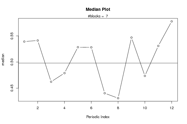
| Title produced by software | Mean Plot | ||||||||||||||||||||
| Date of computation | Wed, 29 Dec 2010 12:13:00 +0000 | ||||||||||||||||||||
| Cite this page as follows | Statistical Computations at FreeStatistics.org, Office for Research Development and Education, URL https://freestatistics.org/blog/index.php?v=date/2010/Dec/29/t1293624650vozqkagdi3gcl40.htm/, Retrieved Fri, 03 May 2024 06:17:29 +0000 | ||||||||||||||||||||
| Statistical Computations at FreeStatistics.org, Office for Research Development and Education, URL https://freestatistics.org/blog/index.php?pk=116739, Retrieved Fri, 03 May 2024 06:17:29 +0000 | |||||||||||||||||||||
| QR Codes: | |||||||||||||||||||||
|
| |||||||||||||||||||||
| Original text written by user: | |||||||||||||||||||||
| IsPrivate? | No (this computation is public) | ||||||||||||||||||||
| User-defined keywords | |||||||||||||||||||||
| Estimated Impact | 168 | ||||||||||||||||||||
Tree of Dependent Computations | |||||||||||||||||||||
| Family? (F = Feedback message, R = changed R code, M = changed R Module, P = changed Parameters, D = changed Data) | |||||||||||||||||||||
| - [Mean Plot] [3/11/2009] [2009-11-02 22:07:54] [b98453cac15ba1066b407e146608df68] - R PD [Mean Plot] [] [2009-12-19 15:08:23] [69c775ce4d55db2aa75a88e773e8d700] - [Mean Plot] [] [2010-12-26 17:09:45] [69c775ce4d55db2aa75a88e773e8d700] - D [Mean Plot] [] [2010-12-29 12:13:00] [e180d4cd19004beeddc12e67012247dc] [Current] | |||||||||||||||||||||
| Feedback Forum | |||||||||||||||||||||
Post a new message | |||||||||||||||||||||
Dataset | |||||||||||||||||||||
| Dataseries X: | |||||||||||||||||||||
00,521505 00,424828 00,425031 00,477194 00,828021 00,615619 00,366627 00,430888 00,281029 00,464625 00,269395 00,577905 00,566115 00,507758 00,750718 00,680840 00,766109 00,456147 00,497750 00,419327 00,609551 00,457337 00,570548 00,347900 00,387499 00,582429 00,239103 00,236745 00,262616 00,424093 00,365275 00,375076 00,409006 00,389168 00,240261 00,158950 00,439337 00,509468 00,374347 00,433983 00,413056 00,328893 00,518665 00,548650 00,546911 00,496349 00,530893 00,595776 00,557058 00,573133 00,500542 00,543127 00,559366 00,691169 00,440349 00,567666 00,596911 00,473554 00,592394 00,597556 00,633413 00,605712 00,704611 00,480526 00,702686 00,700902 00,603085 00,698092 00,597656 00,802342 00,601711 00,599313 00,602563 00,701663 00,499571 00,498092 00,497569 00,600183 00,333954 00,274437 00,320943 00,540667 00,405021 00,288596 00,327594 00,313261 00,257556 00,213839 00,186186 00,159271 | |||||||||||||||||||||
Tables (Output of Computation) | |||||||||||||||||||||
| |||||||||||||||||||||
Figures (Output of Computation) | |||||||||||||||||||||
Input Parameters & R Code | |||||||||||||||||||||
| Parameters (Session): | |||||||||||||||||||||
| par1 = 12 ; | |||||||||||||||||||||
| Parameters (R input): | |||||||||||||||||||||
| par1 = 12 ; | |||||||||||||||||||||
| R code (references can be found in the software module): | |||||||||||||||||||||
par1 <- as.numeric(par1) | |||||||||||||||||||||