Free Statistics
of Irreproducible Research!
Description of Statistical Computation | |||||||||||||||||||||
|---|---|---|---|---|---|---|---|---|---|---|---|---|---|---|---|---|---|---|---|---|---|
| Author's title | |||||||||||||||||||||
| Author | *The author of this computation has been verified* | ||||||||||||||||||||
| R Software Module | rwasp_meanplot.wasp | ||||||||||||||||||||
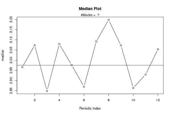
| Title produced by software | Mean Plot | ||||||||||||||||||||
| Date of computation | Wed, 29 Dec 2010 12:11:33 +0000 | ||||||||||||||||||||
| Cite this page as follows | Statistical Computations at FreeStatistics.org, Office for Research Development and Education, URL https://freestatistics.org/blog/index.php?v=date/2010/Dec/29/t1293624557on2dkhs8rxggz10.htm/, Retrieved Fri, 03 May 2024 12:38:25 +0000 | ||||||||||||||||||||
| Statistical Computations at FreeStatistics.org, Office for Research Development and Education, URL https://freestatistics.org/blog/index.php?pk=116737, Retrieved Fri, 03 May 2024 12:38:25 +0000 | |||||||||||||||||||||
| QR Codes: | |||||||||||||||||||||
|
| |||||||||||||||||||||
| Original text written by user: | |||||||||||||||||||||
| IsPrivate? | No (this computation is public) | ||||||||||||||||||||
| User-defined keywords | |||||||||||||||||||||
| Estimated Impact | 167 | ||||||||||||||||||||
Tree of Dependent Computations | |||||||||||||||||||||
| Family? (F = Feedback message, R = changed R code, M = changed R Module, P = changed Parameters, D = changed Data) | |||||||||||||||||||||
| - [Mean Plot] [3/11/2009] [2009-11-02 22:07:54] [b98453cac15ba1066b407e146608df68] - R PD [Mean Plot] [] [2009-12-19 15:08:23] [69c775ce4d55db2aa75a88e773e8d700] - [Mean Plot] [] [2010-12-26 17:09:45] [69c775ce4d55db2aa75a88e773e8d700] - D [Mean Plot] [] [2010-12-29 12:11:33] [e180d4cd19004beeddc12e67012247dc] [Current] | |||||||||||||||||||||
| Feedback Forum | |||||||||||||||||||||
Post a new message | |||||||||||||||||||||
Dataset | |||||||||||||||||||||
| Dataseries X: | |||||||||||||||||||||
04,031636 03,702076 03,056167 03,280707 02,984728 03,693712 03,226317 02,190349 02,599515 03,080288 02,929672 02,922548 03,234943 02,983081 03,284389 03,806511 03,784579 02,645654 03,092081 03,204859 03,107225 03,466909 02,984404 03,218072 02,827310 03,182049 02,236319 02,033218 01,644804 01,627971 01,677559 02,330828 02,493615 02,257172 02,655517 02,298655 02,600402 03,045230 02,790583 03,227052 02,967479 02,938817 03,277961 03,423985 03,072646 02,754253 02,910431 03,174369 03,068387 03,089543 02,906654 02,931161 03,025660 02,939551 02,691019 03,198120 03,076390 02,863873 03,013802 03,053364 02,864753 03,057062 02,959365 03,252258 03,602988 03,497704 03,296867 03,602417 03,300100 03,401930 03,502591 03,402348 03,498551 03,199823 02,700064 02,801034 02,898628 02,800854 02,399942 02,402724 02,202331 02,102594 01,798293 01,202484 01,400201 01,200832 01,298083 01,099742 01,001377 00,836174 | |||||||||||||||||||||
Tables (Output of Computation) | |||||||||||||||||||||
| |||||||||||||||||||||
Figures (Output of Computation) | |||||||||||||||||||||
Input Parameters & R Code | |||||||||||||||||||||
| Parameters (Session): | |||||||||||||||||||||
| par1 = 12 ; | |||||||||||||||||||||
| Parameters (R input): | |||||||||||||||||||||
| par1 = 12 ; | |||||||||||||||||||||
| R code (references can be found in the software module): | |||||||||||||||||||||
par1 <- as.numeric(par1) | |||||||||||||||||||||