Free Statistics
of Irreproducible Research!
Description of Statistical Computation | |||||||||||||||||||||||||||||||||||||||||||||||||||||||||||||||||||||||||||||||||||||||||||||||||||||||||||||||||||||||||||||||||||||||||||||||||||||||||||||||||||||||||||||||||
|---|---|---|---|---|---|---|---|---|---|---|---|---|---|---|---|---|---|---|---|---|---|---|---|---|---|---|---|---|---|---|---|---|---|---|---|---|---|---|---|---|---|---|---|---|---|---|---|---|---|---|---|---|---|---|---|---|---|---|---|---|---|---|---|---|---|---|---|---|---|---|---|---|---|---|---|---|---|---|---|---|---|---|---|---|---|---|---|---|---|---|---|---|---|---|---|---|---|---|---|---|---|---|---|---|---|---|---|---|---|---|---|---|---|---|---|---|---|---|---|---|---|---|---|---|---|---|---|---|---|---|---|---|---|---|---|---|---|---|---|---|---|---|---|---|---|---|---|---|---|---|---|---|---|---|---|---|---|---|---|---|---|---|---|---|---|---|---|---|---|---|---|---|---|---|---|---|---|
| Author's title | |||||||||||||||||||||||||||||||||||||||||||||||||||||||||||||||||||||||||||||||||||||||||||||||||||||||||||||||||||||||||||||||||||||||||||||||||||||||||||||||||||||||||||||||||
| Author | *The author of this computation has been verified* | ||||||||||||||||||||||||||||||||||||||||||||||||||||||||||||||||||||||||||||||||||||||||||||||||||||||||||||||||||||||||||||||||||||||||||||||||||||||||||||||||||||||||||||||||
| R Software Module | rwasp_smp.wasp | ||||||||||||||||||||||||||||||||||||||||||||||||||||||||||||||||||||||||||||||||||||||||||||||||||||||||||||||||||||||||||||||||||||||||||||||||||||||||||||||||||||||||||||||||
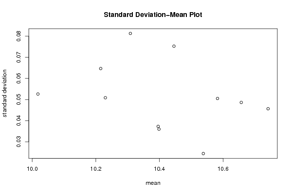
| Title produced by software | Standard Deviation-Mean Plot | ||||||||||||||||||||||||||||||||||||||||||||||||||||||||||||||||||||||||||||||||||||||||||||||||||||||||||||||||||||||||||||||||||||||||||||||||||||||||||||||||||||||||||||||||
| Date of computation | Tue, 28 Dec 2010 14:14:27 +0000 | ||||||||||||||||||||||||||||||||||||||||||||||||||||||||||||||||||||||||||||||||||||||||||||||||||||||||||||||||||||||||||||||||||||||||||||||||||||||||||||||||||||||||||||||||
| Cite this page as follows | Statistical Computations at FreeStatistics.org, Office for Research Development and Education, URL https://freestatistics.org/blog/index.php?v=date/2010/Dec/28/t1293545549ngprmap707cj1ki.htm/, Retrieved Sat, 04 May 2024 23:44:06 +0000 | ||||||||||||||||||||||||||||||||||||||||||||||||||||||||||||||||||||||||||||||||||||||||||||||||||||||||||||||||||||||||||||||||||||||||||||||||||||||||||||||||||||||||||||||||
| Statistical Computations at FreeStatistics.org, Office for Research Development and Education, URL https://freestatistics.org/blog/index.php?pk=116372, Retrieved Sat, 04 May 2024 23:44:06 +0000 | |||||||||||||||||||||||||||||||||||||||||||||||||||||||||||||||||||||||||||||||||||||||||||||||||||||||||||||||||||||||||||||||||||||||||||||||||||||||||||||||||||||||||||||||||
| QR Codes: | |||||||||||||||||||||||||||||||||||||||||||||||||||||||||||||||||||||||||||||||||||||||||||||||||||||||||||||||||||||||||||||||||||||||||||||||||||||||||||||||||||||||||||||||||
|
| |||||||||||||||||||||||||||||||||||||||||||||||||||||||||||||||||||||||||||||||||||||||||||||||||||||||||||||||||||||||||||||||||||||||||||||||||||||||||||||||||||||||||||||||||
| Original text written by user: | |||||||||||||||||||||||||||||||||||||||||||||||||||||||||||||||||||||||||||||||||||||||||||||||||||||||||||||||||||||||||||||||||||||||||||||||||||||||||||||||||||||||||||||||||
| IsPrivate? | No (this computation is public) | ||||||||||||||||||||||||||||||||||||||||||||||||||||||||||||||||||||||||||||||||||||||||||||||||||||||||||||||||||||||||||||||||||||||||||||||||||||||||||||||||||||||||||||||||
| User-defined keywords | |||||||||||||||||||||||||||||||||||||||||||||||||||||||||||||||||||||||||||||||||||||||||||||||||||||||||||||||||||||||||||||||||||||||||||||||||||||||||||||||||||||||||||||||||
| Estimated Impact | 131 | ||||||||||||||||||||||||||||||||||||||||||||||||||||||||||||||||||||||||||||||||||||||||||||||||||||||||||||||||||||||||||||||||||||||||||||||||||||||||||||||||||||||||||||||||
Tree of Dependent Computations | |||||||||||||||||||||||||||||||||||||||||||||||||||||||||||||||||||||||||||||||||||||||||||||||||||||||||||||||||||||||||||||||||||||||||||||||||||||||||||||||||||||||||||||||||
| Family? (F = Feedback message, R = changed R code, M = changed R Module, P = changed Parameters, D = changed Data) | |||||||||||||||||||||||||||||||||||||||||||||||||||||||||||||||||||||||||||||||||||||||||||||||||||||||||||||||||||||||||||||||||||||||||||||||||||||||||||||||||||||||||||||||||
| - [Univariate Data Series] [data set] [2008-12-01 19:54:57] [b98453cac15ba1066b407e146608df68] - RMP [Standard Deviation-Mean Plot] [Unemployment] [2010-11-29 10:34:47] [b98453cac15ba1066b407e146608df68] - PD [Standard Deviation-Mean Plot] [Workshop 6 'Aanta...] [2010-12-14 18:17:59] [40c8b935cbad1b0be3c22a481f9723f7] - R P [Standard Deviation-Mean Plot] [Standard Deviatio...] [2010-12-17 15:30:42] [75b8170d590d2aca2c97c1862bb2167f] - PD [Standard Deviation-Mean Plot] [box-cox] [2010-12-26 11:59:00] [c895532cb7349383dee5125244983cc8] - P [Standard Deviation-Mean Plot] [berekening 14] [2010-12-28 14:14:27] [87bb5e10c18d96bd329dff2d857096c8] [Current] | |||||||||||||||||||||||||||||||||||||||||||||||||||||||||||||||||||||||||||||||||||||||||||||||||||||||||||||||||||||||||||||||||||||||||||||||||||||||||||||||||||||||||||||||||
| Feedback Forum | |||||||||||||||||||||||||||||||||||||||||||||||||||||||||||||||||||||||||||||||||||||||||||||||||||||||||||||||||||||||||||||||||||||||||||||||||||||||||||||||||||||||||||||||||
Post a new message | |||||||||||||||||||||||||||||||||||||||||||||||||||||||||||||||||||||||||||||||||||||||||||||||||||||||||||||||||||||||||||||||||||||||||||||||||||||||||||||||||||||||||||||||||
Dataset | |||||||||||||||||||||||||||||||||||||||||||||||||||||||||||||||||||||||||||||||||||||||||||||||||||||||||||||||||||||||||||||||||||||||||||||||||||||||||||||||||||||||||||||||||
| Dataseries X: | |||||||||||||||||||||||||||||||||||||||||||||||||||||||||||||||||||||||||||||||||||||||||||||||||||||||||||||||||||||||||||||||||||||||||||||||||||||||||||||||||||||||||||||||||
10 10 10 10 10 9,94 10,06 10,06 10,06 10,06 10,06 10,06 10,06 10,06 10,06 10,06 10,06 10,06 10,06 10,06 9,94 9,94 9,94 9,94 9,94 9,94 10,06 10,06 9,94 10,06 10,06 10,06 10,18 10,28 10,28 10,18 10,28 10,28 10,28 10,18 10,28 10,28 10,18 10,18 10,18 10,28 10,28 10,18 10,18 10,18 10,18 10,18 10,18 10,28 10,28 10,28 10,18 10,18 10,18 10,28 10,18 10,18 10,28 10,18 10,18 10,18 10,28 10,28 10,28 10,28 10,28 10,28 10,18 10,18 10,18 10,18 10,18 10,18 10,18 10,18 10,18 10,28 10,28 10,28 10,28 10,28 10,28 10,28 10,28 10,18 10,28 10,28 10,28 10,28 10,18 10,28 10,28 10,28 10,18 10,18 10,28 10,28 10,28 10,28 10,28 10,28 10,28 10,18 10,28 10,28 10,28 10,42 10,42 10,42 10,42 10,42 10,42 10,42 10,42 10,42 10,42 10,34 10,34 10,34 10,42 10,42 10,42 10,42 10,34 10,42 10,42 10,42 10,42 10,42 10,42 10,42 10,42 10,42 10,42 10,42 10,42 10,42 10,42 10,42 10,42 10,42 10,34 10,34 10,34 10,34 10,42 10,42 10,34 10,34 10,34 10,42 10,42 10,42 10,34 10,34 10,34 10,34 10,34 10,42 10,42 10,42 10,34 10,42 10,42 10,42 10,42 10,42 10,42 10,42 10,42 10,42 10,42 10,42 10,42 10,42 10,34 10,34 10,34 10,42 10,42 10,42 10,42 10,42 10,42 10,42 10,42 10,42 10,42 10,42 10,42 10,42 10,42 10,34 10,34 10,42 10,42 10,55 10,55 10,55 10,55 10,55 10,55 10,55 10,55 10,55 10,55 10,49 10,49 10,55 10,55 10,55 10,55 10,55 10,55 10,49 10,55 10,55 10,55 10,55 10,55 10,55 10,49 10,49 10,55 10,55 10,55 10,49 10,55 10,55 10,55 10,55 10,55 10,55 10,55 10,55 10,55 10,49 10,49 10,49 10,55 10,55 10,55 10,49 10,55 10,55 10,55 10,63 10,63 10,63 10,63 10,63 10,57 10,63 10,63 10,63 10,63 10,57 10,57 10,57 10,63 10,63 10,63 10,63 10,57 10,63 10,63 10,57 10,63 10,63 10,63 10,63 10,57 10,63 10,6 10,7 10,7 10,7 10,7 10,7 10,7 10,7 10,7 10,7 10,7 10,6 10,6 10,6 10,6 10,7 10,7 10,6 10,7 10,7 10,7 10,7 10,7 10,7 10,7 10,7 10,7 10,7 10,7 10,7 10,7 10,7 10,8 10,8 10,8 10,8 10,7 10,7 10,7 10,85 10,75 10,75 10,75 10,75 10,75 10,75 10,75 10,75 10,75 10,75 10,75 10,85 10,85 10,85 10,85 10,85 10,85 10,85 10,85 10,85 10,85 10,75 10,75 10,85 10,85 10,85 10,85 10,75 10,75 10,75 10,75 10,75 | |||||||||||||||||||||||||||||||||||||||||||||||||||||||||||||||||||||||||||||||||||||||||||||||||||||||||||||||||||||||||||||||||||||||||||||||||||||||||||||||||||||||||||||||||
Tables (Output of Computation) | |||||||||||||||||||||||||||||||||||||||||||||||||||||||||||||||||||||||||||||||||||||||||||||||||||||||||||||||||||||||||||||||||||||||||||||||||||||||||||||||||||||||||||||||||
| |||||||||||||||||||||||||||||||||||||||||||||||||||||||||||||||||||||||||||||||||||||||||||||||||||||||||||||||||||||||||||||||||||||||||||||||||||||||||||||||||||||||||||||||||
Figures (Output of Computation) | |||||||||||||||||||||||||||||||||||||||||||||||||||||||||||||||||||||||||||||||||||||||||||||||||||||||||||||||||||||||||||||||||||||||||||||||||||||||||||||||||||||||||||||||||
Input Parameters & R Code | |||||||||||||||||||||||||||||||||||||||||||||||||||||||||||||||||||||||||||||||||||||||||||||||||||||||||||||||||||||||||||||||||||||||||||||||||||||||||||||||||||||||||||||||||
| Parameters (Session): | |||||||||||||||||||||||||||||||||||||||||||||||||||||||||||||||||||||||||||||||||||||||||||||||||||||||||||||||||||||||||||||||||||||||||||||||||||||||||||||||||||||||||||||||||
| par1 = 1 ; par2 = 0 ; par3 = 0 ; par4 = 1 ; par5 = 12 ; par6 = White Noise ; par7 = 0.95 ; | |||||||||||||||||||||||||||||||||||||||||||||||||||||||||||||||||||||||||||||||||||||||||||||||||||||||||||||||||||||||||||||||||||||||||||||||||||||||||||||||||||||||||||||||||
| Parameters (R input): | |||||||||||||||||||||||||||||||||||||||||||||||||||||||||||||||||||||||||||||||||||||||||||||||||||||||||||||||||||||||||||||||||||||||||||||||||||||||||||||||||||||||||||||||||
| par1 = 12 ; par2 = 1 ; par3 = 1 ; par4 = 0 ; par5 = 12 ; par6 = White Noise ; par7 = 0.95 ; par8 = ; par9 = ; par10 = ; par11 = ; par12 = ; par13 = ; par14 = ; par15 = ; par16 = ; par17 = ; par18 = ; par19 = ; par20 = ; | |||||||||||||||||||||||||||||||||||||||||||||||||||||||||||||||||||||||||||||||||||||||||||||||||||||||||||||||||||||||||||||||||||||||||||||||||||||||||||||||||||||||||||||||||
| R code (references can be found in the software module): | |||||||||||||||||||||||||||||||||||||||||||||||||||||||||||||||||||||||||||||||||||||||||||||||||||||||||||||||||||||||||||||||||||||||||||||||||||||||||||||||||||||||||||||||||
par1 <- 30 | |||||||||||||||||||||||||||||||||||||||||||||||||||||||||||||||||||||||||||||||||||||||||||||||||||||||||||||||||||||||||||||||||||||||||||||||||||||||||||||||||||||||||||||||||