Repository of Reproducible Computations

Free Statistics

of Irreproducible Research!

Author's title

Author

*The author of this computation has been verified*

R Software Module

rwasp_autocorrelation.wasp

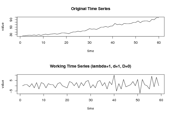
Title produced by software

(Partial) Autocorrelation Function

Date of computation

Mon, 27 Dec 2010 18:56:38 +0000

Cite this page as follows

Statistical Computations at FreeStatistics.org, Office for Research Development and Education, URL https://freestatistics.org/blog/index.php?v=date/2010/Dec/27/t1293476336kij4uk7qvysq7ql.htm/, Retrieved Mon, 06 May 2024 21:10:20 +0000

Statistical Computations at FreeStatistics.org, Office for Research Development and Education, URL https://freestatistics.org/blog/index.php?pk=116086, Retrieved Mon, 06 May 2024 21:10:20 +0000

QR Codes:

Paste this QR Code to cite your computation.

Original text written by user:

IsPrivate?

No (this computation is public)

User-defined keywords

Partial Autocorrelation Function d=1 & D=0 - Gemiddelde bouwgrondprijzen België (1995-2009)

Estimated Impact

117

Family? (F = Feedback message, R = changed R code, M = changed R Module, P = changed Parameters, D = changed Data)

-     [Univariate Data Series] [] [2008-12-08 19:22:39] [d2d412c7f4d35ffbf5ee5ee89db327d4]
- RMPD  [(Partial) Autocorrelation Function] [] [2010-12-14 12:29:39] [42a441ca3193af442aa2201743dfb347]
-    D    [(Partial) Autocorrelation Function] [] [2010-12-14 12:48:13] [43e84bd88d5f94b739fa54f225367516]
- R         [(Partial) Autocorrelation Function] [Partial Autocorre...] [2010-12-17 16:38:22] [78a5cb23fbaf3f7e43a4286844511628]
-   P         [(Partial) Autocorrelation Function] [D=1,d=0] [2010-12-17 17:04:47] [78a5cb23fbaf3f7e43a4286844511628]
-   PD            [(Partial) Autocorrelation Function] [Paper Statistiek] [2010-12-27 18:56:38] [f6fdc0236f011c1845380977efc505f8] [Current]

Feedback Forum

Post a new message

Dataseries X:

Download CSV

Histogram

Boxplots

Summary of computational transaction
Raw Input	view raw input (R code)
Raw Output	view raw output of R engine
Computing time	2 seconds
R Server	'Gwilym Jenkins' @ 72.249.127.135

\begin{tabular}{lllllllll}
\hline
Summary of computational transaction \tabularnewline
Raw Input & view raw input (R code)  \tabularnewline
Raw Output & view raw output of R engine  \tabularnewline
Computing time & 2 seconds \tabularnewline
R Server & 'Gwilym Jenkins' @ 72.249.127.135 \tabularnewline
\hline
\end{tabular}
%Source: https://freestatistics.org/blog/index.php?pk=116086&T=0

[TABLE]
[ROW][C]Summary of computational transaction[/C][/ROW]
[ROW][C]Raw Input[/C][C]view raw input (R code) [/C][/ROW]
[ROW][C]Raw Output[/C][C]view raw output of R engine [/C][/ROW]
[ROW][C]Computing time[/C][C]2 seconds[/C][/ROW]
[ROW][C]R Server[/C][C]'Gwilym Jenkins' @ 72.249.127.135[/C][/ROW]
[/TABLE]
Source: https://freestatistics.org/blog/index.php?pk=116086&T=0

Globally Unique Identifier (entire table): ba.freestatistics.org/blog/index.php?pk=116086&T=0

As an alternative you can also use a QR Code:

The GUIDs for individual cells are displayed in the table below:

Summary of computational transaction
Raw Input	view raw input (R code)
Raw Output	view raw output of R engine
Computing time	2 seconds
R Server	'Gwilym Jenkins' @ 72.249.127.135

Autocorrelation Function
Time lag k	ACF(k)	T-STAT	P-value
1	-0.511599	-3.9297	0.000113
2	0.278825	2.1417	0.018179
3	-0.384231	-2.9513	0.002267
4	0.26893	2.0657	0.021629
5	-0.099955	-0.7678	0.222844
6	0.22652	1.7399	0.043543
7	-0.221804	-1.7037	0.046849
8	0.165329	1.2699	0.10455
9	-0.175952	-1.3515	0.090845
10	0.18587	1.4277	0.079325
11	-0.172221	-1.3229	0.095494
12	0.293973	2.258	0.013828
13	-0.252165	-1.9369	0.028774
14	0.217051	1.6672	0.050388
15	-0.321289	-2.4679	0.008256
16	0.237943	1.8277	0.036328
17	-0.136959	-1.052	0.148544
18	0.12087	0.9284	0.178486
19	0.024058	0.1848	0.427014
20	-0.067844	-0.5211	0.302118
21	-0.058909	-0.4525	0.326289
22	0.044657	0.343	0.366403
23	0.003025	0.0232	0.490769
24	0.095096	0.7304	0.234004
25	-0.129266	-0.9929	0.162403
26	0.025594	0.1966	0.422411
27	-0.008806	-0.0676	0.473151
28	0.019773	0.1519	0.439899
29	-0.031437	-0.2415	0.405012
30	0.017325	0.1331	0.447293
31	0.036163	0.2778	0.391079
32	-0.024411	-0.1875	0.425955
33	-0.030154	-0.2316	0.408817
34	-0.052007	-0.3995	0.345493
35	0.104122	0.7998	0.213525
36	-0.047386	-0.364	0.358588
37	0.036752	0.2823	0.389353
38	-0.074605	-0.573	0.284395
39	-0.005173	-0.0397	0.484219
40	0.047799	0.3671	0.357411
41	-0.018765	-0.1441	0.442941
42	-0.041131	-0.3159	0.376585
43	0.047243	0.3629	0.358995
44	-0.052618	-0.4042	0.343775
45	0.015599	0.1198	0.452517
46	-0.026221	-0.2014	0.420535
47	0.037382	0.2871	0.387507
48	-0.063181	-0.4853	0.314629

\begin{tabular}{lllllllll}
\hline
Autocorrelation Function \tabularnewline
Time lag k & ACF(k) & T-STAT & P-value \tabularnewline
1 & -0.511599 & -3.9297 & 0.000113 \tabularnewline
2 & 0.278825 & 2.1417 & 0.018179 \tabularnewline
3 & -0.384231 & -2.9513 & 0.002267 \tabularnewline
4 & 0.26893 & 2.0657 & 0.021629 \tabularnewline
5 & -0.099955 & -0.7678 & 0.222844 \tabularnewline
6 & 0.22652 & 1.7399 & 0.043543 \tabularnewline
7 & -0.221804 & -1.7037 & 0.046849 \tabularnewline
8 & 0.165329 & 1.2699 & 0.10455 \tabularnewline
9 & -0.175952 & -1.3515 & 0.090845 \tabularnewline
10 & 0.18587 & 1.4277 & 0.079325 \tabularnewline
11 & -0.172221 & -1.3229 & 0.095494 \tabularnewline
12 & 0.293973 & 2.258 & 0.013828 \tabularnewline
13 & -0.252165 & -1.9369 & 0.028774 \tabularnewline
14 & 0.217051 & 1.6672 & 0.050388 \tabularnewline
15 & -0.321289 & -2.4679 & 0.008256 \tabularnewline
16 & 0.237943 & 1.8277 & 0.036328 \tabularnewline
17 & -0.136959 & -1.052 & 0.148544 \tabularnewline
18 & 0.12087 & 0.9284 & 0.178486 \tabularnewline
19 & 0.024058 & 0.1848 & 0.427014 \tabularnewline
20 & -0.067844 & -0.5211 & 0.302118 \tabularnewline
21 & -0.058909 & -0.4525 & 0.326289 \tabularnewline
22 & 0.044657 & 0.343 & 0.366403 \tabularnewline
23 & 0.003025 & 0.0232 & 0.490769 \tabularnewline
24 & 0.095096 & 0.7304 & 0.234004 \tabularnewline
25 & -0.129266 & -0.9929 & 0.162403 \tabularnewline
26 & 0.025594 & 0.1966 & 0.422411 \tabularnewline
27 & -0.008806 & -0.0676 & 0.473151 \tabularnewline
28 & 0.019773 & 0.1519 & 0.439899 \tabularnewline
29 & -0.031437 & -0.2415 & 0.405012 \tabularnewline
30 & 0.017325 & 0.1331 & 0.447293 \tabularnewline
31 & 0.036163 & 0.2778 & 0.391079 \tabularnewline
32 & -0.024411 & -0.1875 & 0.425955 \tabularnewline
33 & -0.030154 & -0.2316 & 0.408817 \tabularnewline
34 & -0.052007 & -0.3995 & 0.345493 \tabularnewline
35 & 0.104122 & 0.7998 & 0.213525 \tabularnewline
36 & -0.047386 & -0.364 & 0.358588 \tabularnewline
37 & 0.036752 & 0.2823 & 0.389353 \tabularnewline
38 & -0.074605 & -0.573 & 0.284395 \tabularnewline
39 & -0.005173 & -0.0397 & 0.484219 \tabularnewline
40 & 0.047799 & 0.3671 & 0.357411 \tabularnewline
41 & -0.018765 & -0.1441 & 0.442941 \tabularnewline
42 & -0.041131 & -0.3159 & 0.376585 \tabularnewline
43 & 0.047243 & 0.3629 & 0.358995 \tabularnewline
44 & -0.052618 & -0.4042 & 0.343775 \tabularnewline
45 & 0.015599 & 0.1198 & 0.452517 \tabularnewline
46 & -0.026221 & -0.2014 & 0.420535 \tabularnewline
47 & 0.037382 & 0.2871 & 0.387507 \tabularnewline
48 & -0.063181 & -0.4853 & 0.314629 \tabularnewline
\hline
\end{tabular}
%Source: https://freestatistics.org/blog/index.php?pk=116086&T=1

[TABLE]
[ROW][C]Autocorrelation Function[/C][/ROW]
[ROW][C]Time lag k[/C][C]ACF(k)[/C][C]T-STAT[/C][C]P-value[/C][/ROW]
[ROW][C]1[/C][C]-0.511599[/C][C]-3.9297[/C][C]0.000113[/C][/ROW]
[ROW][C]2[/C][C]0.278825[/C][C]2.1417[/C][C]0.018179[/C][/ROW]
[ROW][C]3[/C][C]-0.384231[/C][C]-2.9513[/C][C]0.002267[/C][/ROW]
[ROW][C]4[/C][C]0.26893[/C][C]2.0657[/C][C]0.021629[/C][/ROW]
[ROW][C]5[/C][C]-0.099955[/C][C]-0.7678[/C][C]0.222844[/C][/ROW]
[ROW][C]6[/C][C]0.22652[/C][C]1.7399[/C][C]0.043543[/C][/ROW]
[ROW][C]7[/C][C]-0.221804[/C][C]-1.7037[/C][C]0.046849[/C][/ROW]
[ROW][C]8[/C][C]0.165329[/C][C]1.2699[/C][C]0.10455[/C][/ROW]
[ROW][C]9[/C][C]-0.175952[/C][C]-1.3515[/C][C]0.090845[/C][/ROW]
[ROW][C]10[/C][C]0.18587[/C][C]1.4277[/C][C]0.079325[/C][/ROW]
[ROW][C]11[/C][C]-0.172221[/C][C]-1.3229[/C][C]0.095494[/C][/ROW]
[ROW][C]12[/C][C]0.293973[/C][C]2.258[/C][C]0.013828[/C][/ROW]
[ROW][C]13[/C][C]-0.252165[/C][C]-1.9369[/C][C]0.028774[/C][/ROW]
[ROW][C]14[/C][C]0.217051[/C][C]1.6672[/C][C]0.050388[/C][/ROW]
[ROW][C]15[/C][C]-0.321289[/C][C]-2.4679[/C][C]0.008256[/C][/ROW]
[ROW][C]16[/C][C]0.237943[/C][C]1.8277[/C][C]0.036328[/C][/ROW]
[ROW][C]17[/C][C]-0.136959[/C][C]-1.052[/C][C]0.148544[/C][/ROW]
[ROW][C]18[/C][C]0.12087[/C][C]0.9284[/C][C]0.178486[/C][/ROW]
[ROW][C]19[/C][C]0.024058[/C][C]0.1848[/C][C]0.427014[/C][/ROW]
[ROW][C]20[/C][C]-0.067844[/C][C]-0.5211[/C][C]0.302118[/C][/ROW]
[ROW][C]21[/C][C]-0.058909[/C][C]-0.4525[/C][C]0.326289[/C][/ROW]
[ROW][C]22[/C][C]0.044657[/C][C]0.343[/C][C]0.366403[/C][/ROW]
[ROW][C]23[/C][C]0.003025[/C][C]0.0232[/C][C]0.490769[/C][/ROW]
[ROW][C]24[/C][C]0.095096[/C][C]0.7304[/C][C]0.234004[/C][/ROW]
[ROW][C]25[/C][C]-0.129266[/C][C]-0.9929[/C][C]0.162403[/C][/ROW]
[ROW][C]26[/C][C]0.025594[/C][C]0.1966[/C][C]0.422411[/C][/ROW]
[ROW][C]27[/C][C]-0.008806[/C][C]-0.0676[/C][C]0.473151[/C][/ROW]
[ROW][C]28[/C][C]0.019773[/C][C]0.1519[/C][C]0.439899[/C][/ROW]
[ROW][C]29[/C][C]-0.031437[/C][C]-0.2415[/C][C]0.405012[/C][/ROW]
[ROW][C]30[/C][C]0.017325[/C][C]0.1331[/C][C]0.447293[/C][/ROW]
[ROW][C]31[/C][C]0.036163[/C][C]0.2778[/C][C]0.391079[/C][/ROW]
[ROW][C]32[/C][C]-0.024411[/C][C]-0.1875[/C][C]0.425955[/C][/ROW]
[ROW][C]33[/C][C]-0.030154[/C][C]-0.2316[/C][C]0.408817[/C][/ROW]
[ROW][C]34[/C][C]-0.052007[/C][C]-0.3995[/C][C]0.345493[/C][/ROW]
[ROW][C]35[/C][C]0.104122[/C][C]0.7998[/C][C]0.213525[/C][/ROW]
[ROW][C]36[/C][C]-0.047386[/C][C]-0.364[/C][C]0.358588[/C][/ROW]
[ROW][C]37[/C][C]0.036752[/C][C]0.2823[/C][C]0.389353[/C][/ROW]
[ROW][C]38[/C][C]-0.074605[/C][C]-0.573[/C][C]0.284395[/C][/ROW]
[ROW][C]39[/C][C]-0.005173[/C][C]-0.0397[/C][C]0.484219[/C][/ROW]
[ROW][C]40[/C][C]0.047799[/C][C]0.3671[/C][C]0.357411[/C][/ROW]
[ROW][C]41[/C][C]-0.018765[/C][C]-0.1441[/C][C]0.442941[/C][/ROW]
[ROW][C]42[/C][C]-0.041131[/C][C]-0.3159[/C][C]0.376585[/C][/ROW]
[ROW][C]43[/C][C]0.047243[/C][C]0.3629[/C][C]0.358995[/C][/ROW]
[ROW][C]44[/C][C]-0.052618[/C][C]-0.4042[/C][C]0.343775[/C][/ROW]
[ROW][C]45[/C][C]0.015599[/C][C]0.1198[/C][C]0.452517[/C][/ROW]
[ROW][C]46[/C][C]-0.026221[/C][C]-0.2014[/C][C]0.420535[/C][/ROW]
[ROW][C]47[/C][C]0.037382[/C][C]0.2871[/C][C]0.387507[/C][/ROW]
[ROW][C]48[/C][C]-0.063181[/C][C]-0.4853[/C][C]0.314629[/C][/ROW]
[/TABLE]
Source: https://freestatistics.org/blog/index.php?pk=116086&T=1

Globally Unique Identifier (entire table): ba.freestatistics.org/blog/index.php?pk=116086&T=1

As an alternative you can also use a QR Code:

The GUIDs for individual cells are displayed in the table below:

Autocorrelation Function
Time lag k	ACF(k)	T-STAT	P-value
1	-0.511599	-3.9297	0.000113
2	0.278825	2.1417	0.018179
3	-0.384231	-2.9513	0.002267
4	0.26893	2.0657	0.021629
5	-0.099955	-0.7678	0.222844
6	0.22652	1.7399	0.043543
7	-0.221804	-1.7037	0.046849
8	0.165329	1.2699	0.10455
9	-0.175952	-1.3515	0.090845
10	0.18587	1.4277	0.079325
11	-0.172221	-1.3229	0.095494
12	0.293973	2.258	0.013828
13	-0.252165	-1.9369	0.028774
14	0.217051	1.6672	0.050388
15	-0.321289	-2.4679	0.008256
16	0.237943	1.8277	0.036328
17	-0.136959	-1.052	0.148544
18	0.12087	0.9284	0.178486
19	0.024058	0.1848	0.427014
20	-0.067844	-0.5211	0.302118
21	-0.058909	-0.4525	0.326289
22	0.044657	0.343	0.366403
23	0.003025	0.0232	0.490769
24	0.095096	0.7304	0.234004
25	-0.129266	-0.9929	0.162403
26	0.025594	0.1966	0.422411
27	-0.008806	-0.0676	0.473151
28	0.019773	0.1519	0.439899
29	-0.031437	-0.2415	0.405012
30	0.017325	0.1331	0.447293
31	0.036163	0.2778	0.391079
32	-0.024411	-0.1875	0.425955
33	-0.030154	-0.2316	0.408817
34	-0.052007	-0.3995	0.345493
35	0.104122	0.7998	0.213525
36	-0.047386	-0.364	0.358588
37	0.036752	0.2823	0.389353
38	-0.074605	-0.573	0.284395
39	-0.005173	-0.0397	0.484219
40	0.047799	0.3671	0.357411
41	-0.018765	-0.1441	0.442941
42	-0.041131	-0.3159	0.376585
43	0.047243	0.3629	0.358995
44	-0.052618	-0.4042	0.343775
45	0.015599	0.1198	0.452517
46	-0.026221	-0.2014	0.420535
47	0.037382	0.2871	0.387507
48	-0.063181	-0.4853	0.314629

Partial Autocorrelation Function
Time lag k	PACF(k)	T-STAT	P-value
1	-0.511599	-3.9297	0.000113
2	0.023151	0.1778	0.429734
3	-0.315831	-2.4259	0.009173
4	-0.0667	-0.5123	0.305166
5	0.069614	0.5347	0.297427
6	0.185199	1.4225	0.080068
7	0.007709	0.0592	0.476492
8	0.100749	0.7739	0.221049
9	0.010615	0.0815	0.467645
10	0.025751	0.1978	0.421941
11	-0.071409	-0.5485	0.292707
12	0.208713	1.6032	0.05712
13	0.027691	0.2127	0.416148
14	0.067945	0.5219	0.301848
15	-0.13209	-1.0146	0.15722
16	-0.089382	-0.6866	0.247527
17	-0.042422	-0.3258	0.372846
18	-0.148709	-1.1423	0.128981
19	0.22165	1.7025	0.04696
20	-0.001927	-0.0148	0.494119
21	-0.060011	-0.461	0.323264
22	-0.007599	-0.0584	0.476826
23	0.00954	0.0733	0.470917
24	0.00662	0.0508	0.479809
25	-0.053309	-0.4095	0.341837
26	-0.023567	-0.181	0.428486
27	0.132488	1.0177	0.156498
28	-0.078234	-0.6009	0.275095
29	-0.071965	-0.5528	0.291254
30	-0.024712	-0.1898	0.425051
31	0.013603	0.1045	0.45857
32	0.03775	0.29	0.38643
33	-0.056374	-0.433	0.33329
34	0.035138	0.2699	0.394089
35	0.02769	0.2127	0.416151
36	-0.067563	-0.519	0.302865
37	0.029016	0.2229	0.4122
38	-0.029291	-0.225	0.411383
39	-0.057813	-0.4441	0.329308
40	0.060748	0.4666	0.321246
41	-0.036374	-0.2794	0.390459
42	-0.081321	-0.6246	0.267309
43	-0.046728	-0.3589	0.360468
44	0.016755	0.1287	0.449018
45	-0.035212	-0.2705	0.393871
46	-0.053829	-0.4135	0.340381
47	0.062613	0.4809	0.31617
48	-0.04878	-0.3747	0.354618

\begin{tabular}{lllllllll}
\hline
Partial Autocorrelation Function \tabularnewline
Time lag k & PACF(k) & T-STAT & P-value \tabularnewline
1 & -0.511599 & -3.9297 & 0.000113 \tabularnewline
2 & 0.023151 & 0.1778 & 0.429734 \tabularnewline
3 & -0.315831 & -2.4259 & 0.009173 \tabularnewline
4 & -0.0667 & -0.5123 & 0.305166 \tabularnewline
5 & 0.069614 & 0.5347 & 0.297427 \tabularnewline
6 & 0.185199 & 1.4225 & 0.080068 \tabularnewline
7 & 0.007709 & 0.0592 & 0.476492 \tabularnewline
8 & 0.100749 & 0.7739 & 0.221049 \tabularnewline
9 & 0.010615 & 0.0815 & 0.467645 \tabularnewline
10 & 0.025751 & 0.1978 & 0.421941 \tabularnewline
11 & -0.071409 & -0.5485 & 0.292707 \tabularnewline
12 & 0.208713 & 1.6032 & 0.05712 \tabularnewline
13 & 0.027691 & 0.2127 & 0.416148 \tabularnewline
14 & 0.067945 & 0.5219 & 0.301848 \tabularnewline
15 & -0.13209 & -1.0146 & 0.15722 \tabularnewline
16 & -0.089382 & -0.6866 & 0.247527 \tabularnewline
17 & -0.042422 & -0.3258 & 0.372846 \tabularnewline
18 & -0.148709 & -1.1423 & 0.128981 \tabularnewline
19 & 0.22165 & 1.7025 & 0.04696 \tabularnewline
20 & -0.001927 & -0.0148 & 0.494119 \tabularnewline
21 & -0.060011 & -0.461 & 0.323264 \tabularnewline
22 & -0.007599 & -0.0584 & 0.476826 \tabularnewline
23 & 0.00954 & 0.0733 & 0.470917 \tabularnewline
24 & 0.00662 & 0.0508 & 0.479809 \tabularnewline
25 & -0.053309 & -0.4095 & 0.341837 \tabularnewline
26 & -0.023567 & -0.181 & 0.428486 \tabularnewline
27 & 0.132488 & 1.0177 & 0.156498 \tabularnewline
28 & -0.078234 & -0.6009 & 0.275095 \tabularnewline
29 & -0.071965 & -0.5528 & 0.291254 \tabularnewline
30 & -0.024712 & -0.1898 & 0.425051 \tabularnewline
31 & 0.013603 & 0.1045 & 0.45857 \tabularnewline
32 & 0.03775 & 0.29 & 0.38643 \tabularnewline
33 & -0.056374 & -0.433 & 0.33329 \tabularnewline
34 & 0.035138 & 0.2699 & 0.394089 \tabularnewline
35 & 0.02769 & 0.2127 & 0.416151 \tabularnewline
36 & -0.067563 & -0.519 & 0.302865 \tabularnewline
37 & 0.029016 & 0.2229 & 0.4122 \tabularnewline
38 & -0.029291 & -0.225 & 0.411383 \tabularnewline
39 & -0.057813 & -0.4441 & 0.329308 \tabularnewline
40 & 0.060748 & 0.4666 & 0.321246 \tabularnewline
41 & -0.036374 & -0.2794 & 0.390459 \tabularnewline
42 & -0.081321 & -0.6246 & 0.267309 \tabularnewline
43 & -0.046728 & -0.3589 & 0.360468 \tabularnewline
44 & 0.016755 & 0.1287 & 0.449018 \tabularnewline
45 & -0.035212 & -0.2705 & 0.393871 \tabularnewline
46 & -0.053829 & -0.4135 & 0.340381 \tabularnewline
47 & 0.062613 & 0.4809 & 0.31617 \tabularnewline
48 & -0.04878 & -0.3747 & 0.354618 \tabularnewline
\hline
\end{tabular}
%Source: https://freestatistics.org/blog/index.php?pk=116086&T=2

[TABLE]
[ROW][C]Partial Autocorrelation Function[/C][/ROW]
[ROW][C]Time lag k[/C][C]PACF(k)[/C][C]T-STAT[/C][C]P-value[/C][/ROW]
[ROW][C]1[/C][C]-0.511599[/C][C]-3.9297[/C][C]0.000113[/C][/ROW]
[ROW][C]2[/C][C]0.023151[/C][C]0.1778[/C][C]0.429734[/C][/ROW]
[ROW][C]3[/C][C]-0.315831[/C][C]-2.4259[/C][C]0.009173[/C][/ROW]
[ROW][C]4[/C][C]-0.0667[/C][C]-0.5123[/C][C]0.305166[/C][/ROW]
[ROW][C]5[/C][C]0.069614[/C][C]0.5347[/C][C]0.297427[/C][/ROW]
[ROW][C]6[/C][C]0.185199[/C][C]1.4225[/C][C]0.080068[/C][/ROW]
[ROW][C]7[/C][C]0.007709[/C][C]0.0592[/C][C]0.476492[/C][/ROW]
[ROW][C]8[/C][C]0.100749[/C][C]0.7739[/C][C]0.221049[/C][/ROW]
[ROW][C]9[/C][C]0.010615[/C][C]0.0815[/C][C]0.467645[/C][/ROW]
[ROW][C]10[/C][C]0.025751[/C][C]0.1978[/C][C]0.421941[/C][/ROW]
[ROW][C]11[/C][C]-0.071409[/C][C]-0.5485[/C][C]0.292707[/C][/ROW]
[ROW][C]12[/C][C]0.208713[/C][C]1.6032[/C][C]0.05712[/C][/ROW]
[ROW][C]13[/C][C]0.027691[/C][C]0.2127[/C][C]0.416148[/C][/ROW]
[ROW][C]14[/C][C]0.067945[/C][C]0.5219[/C][C]0.301848[/C][/ROW]
[ROW][C]15[/C][C]-0.13209[/C][C]-1.0146[/C][C]0.15722[/C][/ROW]
[ROW][C]16[/C][C]-0.089382[/C][C]-0.6866[/C][C]0.247527[/C][/ROW]
[ROW][C]17[/C][C]-0.042422[/C][C]-0.3258[/C][C]0.372846[/C][/ROW]
[ROW][C]18[/C][C]-0.148709[/C][C]-1.1423[/C][C]0.128981[/C][/ROW]
[ROW][C]19[/C][C]0.22165[/C][C]1.7025[/C][C]0.04696[/C][/ROW]
[ROW][C]20[/C][C]-0.001927[/C][C]-0.0148[/C][C]0.494119[/C][/ROW]
[ROW][C]21[/C][C]-0.060011[/C][C]-0.461[/C][C]0.323264[/C][/ROW]
[ROW][C]22[/C][C]-0.007599[/C][C]-0.0584[/C][C]0.476826[/C][/ROW]
[ROW][C]23[/C][C]0.00954[/C][C]0.0733[/C][C]0.470917[/C][/ROW]
[ROW][C]24[/C][C]0.00662[/C][C]0.0508[/C][C]0.479809[/C][/ROW]
[ROW][C]25[/C][C]-0.053309[/C][C]-0.4095[/C][C]0.341837[/C][/ROW]
[ROW][C]26[/C][C]-0.023567[/C][C]-0.181[/C][C]0.428486[/C][/ROW]
[ROW][C]27[/C][C]0.132488[/C][C]1.0177[/C][C]0.156498[/C][/ROW]
[ROW][C]28[/C][C]-0.078234[/C][C]-0.6009[/C][C]0.275095[/C][/ROW]
[ROW][C]29[/C][C]-0.071965[/C][C]-0.5528[/C][C]0.291254[/C][/ROW]
[ROW][C]30[/C][C]-0.024712[/C][C]-0.1898[/C][C]0.425051[/C][/ROW]
[ROW][C]31[/C][C]0.013603[/C][C]0.1045[/C][C]0.45857[/C][/ROW]
[ROW][C]32[/C][C]0.03775[/C][C]0.29[/C][C]0.38643[/C][/ROW]
[ROW][C]33[/C][C]-0.056374[/C][C]-0.433[/C][C]0.33329[/C][/ROW]
[ROW][C]34[/C][C]0.035138[/C][C]0.2699[/C][C]0.394089[/C][/ROW]
[ROW][C]35[/C][C]0.02769[/C][C]0.2127[/C][C]0.416151[/C][/ROW]
[ROW][C]36[/C][C]-0.067563[/C][C]-0.519[/C][C]0.302865[/C][/ROW]
[ROW][C]37[/C][C]0.029016[/C][C]0.2229[/C][C]0.4122[/C][/ROW]
[ROW][C]38[/C][C]-0.029291[/C][C]-0.225[/C][C]0.411383[/C][/ROW]
[ROW][C]39[/C][C]-0.057813[/C][C]-0.4441[/C][C]0.329308[/C][/ROW]
[ROW][C]40[/C][C]0.060748[/C][C]0.4666[/C][C]0.321246[/C][/ROW]
[ROW][C]41[/C][C]-0.036374[/C][C]-0.2794[/C][C]0.390459[/C][/ROW]
[ROW][C]42[/C][C]-0.081321[/C][C]-0.6246[/C][C]0.267309[/C][/ROW]
[ROW][C]43[/C][C]-0.046728[/C][C]-0.3589[/C][C]0.360468[/C][/ROW]
[ROW][C]44[/C][C]0.016755[/C][C]0.1287[/C][C]0.449018[/C][/ROW]
[ROW][C]45[/C][C]-0.035212[/C][C]-0.2705[/C][C]0.393871[/C][/ROW]
[ROW][C]46[/C][C]-0.053829[/C][C]-0.4135[/C][C]0.340381[/C][/ROW]
[ROW][C]47[/C][C]0.062613[/C][C]0.4809[/C][C]0.31617[/C][/ROW]
[ROW][C]48[/C][C]-0.04878[/C][C]-0.3747[/C][C]0.354618[/C][/ROW]
[/TABLE]
Source: https://freestatistics.org/blog/index.php?pk=116086&T=2

Globally Unique Identifier (entire table): ba.freestatistics.org/blog/index.php?pk=116086&T=2

As an alternative you can also use a QR Code:

The GUIDs for individual cells are displayed in the table below:

Partial Autocorrelation Function
Time lag k	PACF(k)	T-STAT	P-value
1	-0.511599	-3.9297	0.000113
2	0.023151	0.1778	0.429734
3	-0.315831	-2.4259	0.009173
4	-0.0667	-0.5123	0.305166
5	0.069614	0.5347	0.297427
6	0.185199	1.4225	0.080068
7	0.007709	0.0592	0.476492
8	0.100749	0.7739	0.221049
9	0.010615	0.0815	0.467645
10	0.025751	0.1978	0.421941
11	-0.071409	-0.5485	0.292707
12	0.208713	1.6032	0.05712
13	0.027691	0.2127	0.416148
14	0.067945	0.5219	0.301848
15	-0.13209	-1.0146	0.15722
16	-0.089382	-0.6866	0.247527
17	-0.042422	-0.3258	0.372846
18	-0.148709	-1.1423	0.128981
19	0.22165	1.7025	0.04696
20	-0.001927	-0.0148	0.494119
21	-0.060011	-0.461	0.323264
22	-0.007599	-0.0584	0.476826
23	0.00954	0.0733	0.470917
24	0.00662	0.0508	0.479809
25	-0.053309	-0.4095	0.341837
26	-0.023567	-0.181	0.428486
27	0.132488	1.0177	0.156498
28	-0.078234	-0.6009	0.275095
29	-0.071965	-0.5528	0.291254
30	-0.024712	-0.1898	0.425051
31	0.013603	0.1045	0.45857
32	0.03775	0.29	0.38643
33	-0.056374	-0.433	0.33329
34	0.035138	0.2699	0.394089
35	0.02769	0.2127	0.416151
36	-0.067563	-0.519	0.302865
37	0.029016	0.2229	0.4122
38	-0.029291	-0.225	0.411383
39	-0.057813	-0.4441	0.329308
40	0.060748	0.4666	0.321246
41	-0.036374	-0.2794	0.390459
42	-0.081321	-0.6246	0.267309
43	-0.046728	-0.3589	0.360468
44	0.016755	0.1287	0.449018
45	-0.035212	-0.2705	0.393871
46	-0.053829	-0.4135	0.340381
47	0.062613	0.4809	0.31617
48	-0.04878	-0.3747	0.354618

Figure 1

PNG link

Postscript link

PDF link

Figure 2

PNG link

Postscript link

PDF link

Figure 3

PNG link

Postscript link

PDF link

Parameters (Session):

par1 = 48 ; par2 = 1 ; par3 = 1 ; par4 = 0 ; par5 = 4 ; par6 = White Noise ; par7 = 0.95 ;

Parameters (R input):

par1 = 48 ; par2 = 1 ; par3 = 1 ; par4 = 0 ; par5 = 4 ; par6 = White Noise ; par7 = 0.95 ; par8 = ;

R code (references can be found in the software module):

if (par1 == 'Default') {
par1 = 10*log10(length(x))
} else {
par1 <- as.numeric(par1)
}
par2 <- as.numeric(par2)
par3 <- as.numeric(par3)
par4 <- as.numeric(par4)
par5 <- as.numeric(par5)
if (par6 == 'White Noise') par6 <- 'white' else par6 <- 'ma'
par7 <- as.numeric(par7)
if (par8 != '') par8 <- as.numeric(par8)
ox <- x
if (par8 == '') {
if (par2 == 0) {
x <- log(x)
} else {
x <- (x ^ par2 - 1) / par2
}
} else {
x <- log(x,base=par8)
}
if (par3 > 0) x <- diff(x,lag=1,difference=par3)
if (par4 > 0) x <- diff(x,lag=par5,difference=par4)
bitmap(file='picts.png')
op <- par(mfrow=c(2,1))
plot(ox,type='l',main='Original Time Series',xlab='time',ylab='value')
if (par8=='') {
mytitle <- paste('Working Time Series (lambda=',par2,', d=',par3,', D=',par4,')',sep='')
mysub <- paste('(lambda=',par2,', d=',par3,', D=',par4,', CI=', par7, ', CI type=',par6,')',sep='')
} else {
mytitle <- paste('Working Time Series (base=',par8,', d=',par3,', D=',par4,')',sep='')
mysub <- paste('(base=',par8,', d=',par3,', D=',par4,', CI=', par7, ', CI type=',par6,')',sep='')
}
plot(x,type='l', main=mytitle,xlab='time',ylab='value')
par(op)
dev.off()
bitmap(file='pic1.png')
racf <- acf(x, par1, main='Autocorrelation', xlab='time lag', ylab='ACF', ci.type=par6, ci=par7, sub=mysub)
dev.off()
bitmap(file='pic2.png')
rpacf <- pacf(x,par1,main='Partial Autocorrelation',xlab='lags',ylab='PACF',sub=mysub)
dev.off()
(myacf <- c(racf$acf))
(mypacf <- c(rpacf$acf))
lengthx <- length(x)
sqrtn <- sqrt(lengthx)
load(file='createtable')
a<-table.start()
a<-table.row.start(a)
a<-table.element(a,'Autocorrelation Function',4,TRUE)
a<-table.row.end(a)
a<-table.row.start(a)
a<-table.element(a,'Time lag k',header=TRUE)
a<-table.element(a,hyperlink('basics.htm','ACF(k)','click here for more information about the Autocorrelation Function'),header=TRUE)
a<-table.element(a,'T-STAT',header=TRUE)
a<-table.element(a,'P-value',header=TRUE)
a<-table.row.end(a)
for (i in 2:(par1+1)) {
a<-table.row.start(a)
a<-table.element(a,i-1,header=TRUE)
a<-table.element(a,round(myacf[i],6))
mytstat <- myacf[i]*sqrtn
a<-table.element(a,round(mytstat,4))
a<-table.element(a,round(1-pt(abs(mytstat),lengthx),6))
a<-table.row.end(a)
}
a<-table.end(a)
table.save(a,file='mytable.tab')
a<-table.start()
a<-table.row.start(a)
a<-table.element(a,'Partial Autocorrelation Function',4,TRUE)
a<-table.row.end(a)
a<-table.row.start(a)
a<-table.element(a,'Time lag k',header=TRUE)
a<-table.element(a,hyperlink('basics.htm','PACF(k)','click here for more information about the Partial Autocorrelation Function'),header=TRUE)
a<-table.element(a,'T-STAT',header=TRUE)
a<-table.element(a,'P-value',header=TRUE)
a<-table.row.end(a)
for (i in 1:par1) {
a<-table.row.start(a)
a<-table.element(a,i,header=TRUE)
a<-table.element(a,round(mypacf[i],6))
mytstat <- mypacf[i]*sqrtn
a<-table.element(a,round(mytstat,4))
a<-table.element(a,round(1-pt(abs(mytstat),lengthx),6))
a<-table.row.end(a)
}
a<-table.end(a)
table.save(a,file='mytable1.tab')

Free Statistics

Description of Statistical Computation

Tree of Dependent Computations

Dataset

Tables (Output of Computation)

Figures (Output of Computation)

Input Parameters & R Code