Free Statistics
of Irreproducible Research!
Description of Statistical Computation | |||||||||||||||||||||||||||||||||||||||||||||||||||||||||||||||||||||||||||||||||||||||||||||||||||||||||||||||||||||||||||||||||||||||||||||||||||||||||||||||||||||||||
|---|---|---|---|---|---|---|---|---|---|---|---|---|---|---|---|---|---|---|---|---|---|---|---|---|---|---|---|---|---|---|---|---|---|---|---|---|---|---|---|---|---|---|---|---|---|---|---|---|---|---|---|---|---|---|---|---|---|---|---|---|---|---|---|---|---|---|---|---|---|---|---|---|---|---|---|---|---|---|---|---|---|---|---|---|---|---|---|---|---|---|---|---|---|---|---|---|---|---|---|---|---|---|---|---|---|---|---|---|---|---|---|---|---|---|---|---|---|---|---|---|---|---|---|---|---|---|---|---|---|---|---|---|---|---|---|---|---|---|---|---|---|---|---|---|---|---|---|---|---|---|---|---|---|---|---|---|---|---|---|---|---|---|---|---|---|---|---|---|---|
| Author's title | |||||||||||||||||||||||||||||||||||||||||||||||||||||||||||||||||||||||||||||||||||||||||||||||||||||||||||||||||||||||||||||||||||||||||||||||||||||||||||||||||||||||||
| Author | *The author of this computation has been verified* | ||||||||||||||||||||||||||||||||||||||||||||||||||||||||||||||||||||||||||||||||||||||||||||||||||||||||||||||||||||||||||||||||||||||||||||||||||||||||||||||||||||||||
| R Software Module | rwasp_twosampletests_mean.wasp | ||||||||||||||||||||||||||||||||||||||||||||||||||||||||||||||||||||||||||||||||||||||||||||||||||||||||||||||||||||||||||||||||||||||||||||||||||||||||||||||||||||||||
| Title produced by software | Paired and Unpaired Two Samples Tests about the Mean | ||||||||||||||||||||||||||||||||||||||||||||||||||||||||||||||||||||||||||||||||||||||||||||||||||||||||||||||||||||||||||||||||||||||||||||||||||||||||||||||||||||||||
| Date of computation | Sat, 25 Dec 2010 11:18:55 +0000 | ||||||||||||||||||||||||||||||||||||||||||||||||||||||||||||||||||||||||||||||||||||||||||||||||||||||||||||||||||||||||||||||||||||||||||||||||||||||||||||||||||||||||
| Cite this page as follows | Statistical Computations at FreeStatistics.org, Office for Research Development and Education, URL https://freestatistics.org/blog/index.php?v=date/2010/Dec/25/t12932787200h1ifmeqoqmu3fo.htm/, Retrieved Mon, 29 Apr 2024 01:44:38 +0000 | ||||||||||||||||||||||||||||||||||||||||||||||||||||||||||||||||||||||||||||||||||||||||||||||||||||||||||||||||||||||||||||||||||||||||||||||||||||||||||||||||||||||||
| Statistical Computations at FreeStatistics.org, Office for Research Development and Education, URL https://freestatistics.org/blog/index.php?pk=115366, Retrieved Mon, 29 Apr 2024 01:44:38 +0000 | |||||||||||||||||||||||||||||||||||||||||||||||||||||||||||||||||||||||||||||||||||||||||||||||||||||||||||||||||||||||||||||||||||||||||||||||||||||||||||||||||||||||||
| QR Codes: | |||||||||||||||||||||||||||||||||||||||||||||||||||||||||||||||||||||||||||||||||||||||||||||||||||||||||||||||||||||||||||||||||||||||||||||||||||||||||||||||||||||||||
|
| |||||||||||||||||||||||||||||||||||||||||||||||||||||||||||||||||||||||||||||||||||||||||||||||||||||||||||||||||||||||||||||||||||||||||||||||||||||||||||||||||||||||||
| Original text written by user: | |||||||||||||||||||||||||||||||||||||||||||||||||||||||||||||||||||||||||||||||||||||||||||||||||||||||||||||||||||||||||||||||||||||||||||||||||||||||||||||||||||||||||
| IsPrivate? | No (this computation is public) | ||||||||||||||||||||||||||||||||||||||||||||||||||||||||||||||||||||||||||||||||||||||||||||||||||||||||||||||||||||||||||||||||||||||||||||||||||||||||||||||||||||||||
| User-defined keywords | |||||||||||||||||||||||||||||||||||||||||||||||||||||||||||||||||||||||||||||||||||||||||||||||||||||||||||||||||||||||||||||||||||||||||||||||||||||||||||||||||||||||||
| Estimated Impact | 180 | ||||||||||||||||||||||||||||||||||||||||||||||||||||||||||||||||||||||||||||||||||||||||||||||||||||||||||||||||||||||||||||||||||||||||||||||||||||||||||||||||||||||||
Tree of Dependent Computations | |||||||||||||||||||||||||||||||||||||||||||||||||||||||||||||||||||||||||||||||||||||||||||||||||||||||||||||||||||||||||||||||||||||||||||||||||||||||||||||||||||||||||
| Family? (F = Feedback message, R = changed R code, M = changed R Module, P = changed Parameters, D = changed Data) | |||||||||||||||||||||||||||||||||||||||||||||||||||||||||||||||||||||||||||||||||||||||||||||||||||||||||||||||||||||||||||||||||||||||||||||||||||||||||||||||||||||||||
| - [Paired and Unpaired Two Samples Tests about the Mean] [] [2010-11-17 12:33:27] [e45804683e9a4263debf179d74e04a01] - PD [Paired and Unpaired Two Samples Tests about the Mean] [] [2010-12-25 11:18:55] [82d760768aff8bf374d9817688c406af] [Current] - P [Paired and Unpaired Two Samples Tests about the Mean] [test] [2010-12-26 17:25:41] [d6e648f00513dd750579ba7880c5fbf5] - PD [Paired and Unpaired Two Samples Tests about the Mean] [Anova intrinsieke...] [2010-12-27 14:09:55] [d6e648f00513dd750579ba7880c5fbf5] - D [Paired and Unpaired Two Samples Tests about the Mean] [Anova intrinsieke...] [2010-12-27 14:17:58] [d6e648f00513dd750579ba7880c5fbf5] - D [Paired and Unpaired Two Samples Tests about the Mean] [Anova intrinsieke...] [2010-12-27 14:26:46] [d6e648f00513dd750579ba7880c5fbf5] - RMPD [Kendall tau Correlation Matrix] [pearson intrinsiek] [2010-12-27 15:34:42] [d6e648f00513dd750579ba7880c5fbf5] - RMPD [Kendall tau Correlation Matrix] [kendall intrinsiek] [2010-12-27 15:39:32] [d6e648f00513dd750579ba7880c5fbf5] - PD [Paired and Unpaired Two Samples Tests about the Mean] [] [2010-12-27 14:10:54] [e45804683e9a4263debf179d74e04a01] - PD [Paired and Unpaired Two Samples Tests about the Mean] [] [2010-12-27 14:22:38] [e45804683e9a4263debf179d74e04a01] | |||||||||||||||||||||||||||||||||||||||||||||||||||||||||||||||||||||||||||||||||||||||||||||||||||||||||||||||||||||||||||||||||||||||||||||||||||||||||||||||||||||||||
| Feedback Forum | |||||||||||||||||||||||||||||||||||||||||||||||||||||||||||||||||||||||||||||||||||||||||||||||||||||||||||||||||||||||||||||||||||||||||||||||||||||||||||||||||||||||||
Post a new message | |||||||||||||||||||||||||||||||||||||||||||||||||||||||||||||||||||||||||||||||||||||||||||||||||||||||||||||||||||||||||||||||||||||||||||||||||||||||||||||||||||||||||
Dataset | |||||||||||||||||||||||||||||||||||||||||||||||||||||||||||||||||||||||||||||||||||||||||||||||||||||||||||||||||||||||||||||||||||||||||||||||||||||||||||||||||||||||||
| Dataseries X: | |||||||||||||||||||||||||||||||||||||||||||||||||||||||||||||||||||||||||||||||||||||||||||||||||||||||||||||||||||||||||||||||||||||||||||||||||||||||||||||||||||||||||
4 1 27 5 26 49 35 4 1 36 4 25 45 34 5 1 25 4 17 54 13 2 1 27 3 37 36 35 3 2 25 3 35 36 28 5 2 44 3 15 53 32 4 1 50 4 27 46 35 4 1 41 4 36 42 36 4 1 48 5 25 41 27 4 2 43 4 30 45 29 5 2 47 2 27 47 27 4 2 41 3 33 42 28 3 1 44 2 29 45 29 4 2 47 5 30 40 28 3 2 40 3 25 45 30 3 2 46 3 23 40 25 4 1 28 3 26 42 15 3 1 56 3 24 45 33 4 2 49 4 35 47 31 2 2 25 4 39 31 37 4 2 41 4 23 46 37 3 2 26 3 32 34 34 4 1 50 5 29 43 32 4 1 47 4 26 45 21 3 1 52 2 21 42 25 3 2 37 5 35 51 32 2 2 41 3 23 44 28 4 1 45 4 21 47 22 5 2 26 4 28 47 25 4 1 NA 3 30 41 26 2 1 52 4 21 44 34 5 1 46 2 29 51 34 4 1 58 3 28 46 36 3 1 54 5 19 47 36 4 1 29 3 26 46 26 2 2 50 3 33 38 26 3 1 43 2 34 50 34 3 2 30 3 33 48 33 3 2 47 2 40 36 31 5 1 45 3 24 51 33 NA 2 48 1 35 35 22 4 2 48 3 35 49 29 4 2 26 4 32 38 24 4 1 46 5 20 47 37 2 2 NA 3 35 36 32 4 2 50 3 35 47 23 3 1 25 4 21 46 29 4 1 47 2 33 43 35 1 2 47 2 40 53 20 2 1 41 3 22 55 28 2 2 45 2 35 39 26 4 2 41 4 20 55 36 3 2 45 5 28 41 26 4 2 40 3 46 33 33 3 1 29 4 18 52 25 3 2 34 5 22 42 29 5 1 45 5 20 56 32 3 2 52 3 25 46 35 2 2 41 4 31 33 24 1 2 48 3 21 51 31 2 2 45 3 23 46 29 5 1 54 2 26 46 27 4 2 25 3 34 50 29 4 2 26 4 31 46 29 3 1 28 4 23 51 27 4 2 50 4 31 48 34 4 2 48 4 26 44 32 2 2 51 3 36 38 31 3 2 53 3 28 42 31 4 1 37 3 34 39 31 3 1 56 2 25 45 16 2 1 43 3 33 31 25 4 1 34 3 46 29 27 4 1 42 3 24 48 32 3 2 32 3 32 38 28 5 2 31 5 33 55 25 1 1 46 3 42 32 25 3 2 30 5 17 51 36 3 2 47 4 36 53 36 5 2 33 4 40 47 36 2 1 25 4 30 45 27 3 1 25 5 19 33 29 3 2 21 4 33 49 32 4 2 36 5 35 46 29 2 2 50 3 23 42 31 4 2 48 3 15 56 34 3 2 48 2 38 35 27 3 1 25 3 37 40 28 3 1 48 4 23 44 32 2 2 49 5 41 46 33 3 1 27 5 34 46 29 2 1 28 3 38 39 32 4 2 43 2 45 35 35 4 2 48 3 27 48 33 2 2 48 4 46 42 27 1 1 25 1 26 39 16 5 2 49 4 44 39 32 4 1 26 3 36 41 26 4 1 51 3 20 52 32 4 2 25 4 44 45 38 3 1 29 3 27 42 24 3 1 29 4 27 44 26 1 1 43 2 41 33 19 5 2 46 3 30 42 37 3 1 44 3 33 46 25 3 1 25 3 37 45 24 2 1 51 2 30 40 23 4 1 42 5 20 48 28 4 2 53 5 44 32 38 3 1 25 4 20 53 28 4 2 49 2 33 39 28 4 1 51 3 31 45 26 2 2 20 3 23 36 21 3 2 44 3 33 38 35 3 2 38 4 33 49 31 3 1 46 5 32 46 34 4 2 42 4 25 43 30 5 1 29 NA 22 37 30 3 2 46 4 16 48 24 3 2 49 2 36 45 27 2 2 51 3 35 32 26 3 1 38 3 25 46 30 1 1 41 1 27 20 15 4 2 47 3 32 42 28 4 2 44 3 36 45 34 4 2 47 3 51 29 29 3 2 46 3 30 51 26 5 1 44 4 20 55 31 2 2 28 3 29 50 28 2 2 47 4 26 44 33 3 2 28 4 20 41 32 3 1 41 5 40 40 33 2 2 45 4 29 47 31 1 2 46 4 32 42 37 3 1 46 4 33 40 27 5 2 22 3 32 51 19 4 2 33 3 34 43 27 4 1 41 4 24 45 31 4 2 47 5 25 41 38 3 1 25 3 41 41 22 5 2 42 3 39 37 35 3 2 47 3 21 46 35 3 2 50 3 38 38 30 3 1 55 5 28 39 41 3 1 21 3 37 45 25 4 1 NA 3 26 46 28 2 1 52 3 30 39 45 2 2 49 4 25 21 21 4 2 46 4 38 31 33 3 1 NA 4 31 35 25 3 2 45 3 31 49 29 2 2 52 3 27 40 31 3 1 NA 3 21 45 29 3 2 40 4 26 46 31 4 2 49 4 37 45 31 1 1 38 5 28 34 25 1 1 32 5 29 41 27 5 2 46 4 33 43 26 4 2 32 3 41 45 26 3 2 41 3 19 48 23 3 2 43 3 37 43 27 4 1 44 4 36 45 24 3 1 47 5 27 45 35 2 2 28 3 33 34 24 1 1 52 1 29 40 32 1 1 27 2 42 40 24 5 2 45 5 27 55 24 4 1 27 4 47 44 38 3 1 25 4 17 44 36 4 1 28 4 34 48 24 5 1 25 3 32 51 18 4 1 52 4 25 49 34 4 1 44 3 27 33 23 2 2 43 3 37 43 35 3 2 47 4 34 44 22 4 2 52 4 27 44 34 3 2 40 2 37 41 28 4 1 42 3 32 45 34 3 1 45 5 26 44 32 4 1 45 2 29 44 24 1 1 50 5 28 40 34 2 1 49 3 19 48 33 3 1 52 2 46 49 33 3 2 48 3 31 46 29 5 2 51 3 42 49 38 4 2 49 4 33 55 24 3 2 31 4 39 51 25 3 2 43 3 27 46 37 3 2 31 3 35 37 33 3 2 28 4 23 43 30 4 2 43 4 32 41 22 3 2 31 3 22 45 28 2 2 51 3 17 39 24 4 2 58 4 35 38 33 2 2 25 5 34 41 37 | |||||||||||||||||||||||||||||||||||||||||||||||||||||||||||||||||||||||||||||||||||||||||||||||||||||||||||||||||||||||||||||||||||||||||||||||||||||||||||||||||||||||||
Tables (Output of Computation) | |||||||||||||||||||||||||||||||||||||||||||||||||||||||||||||||||||||||||||||||||||||||||||||||||||||||||||||||||||||||||||||||||||||||||||||||||||||||||||||||||||||||||
| |||||||||||||||||||||||||||||||||||||||||||||||||||||||||||||||||||||||||||||||||||||||||||||||||||||||||||||||||||||||||||||||||||||||||||||||||||||||||||||||||||||||||
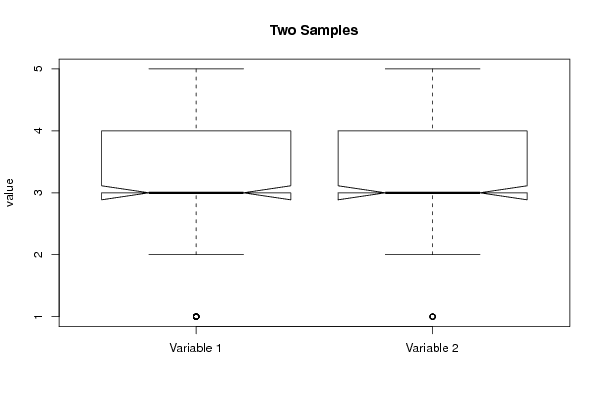
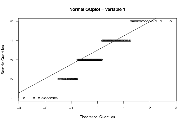
Figures (Output of Computation) | |||||||||||||||||||||||||||||||||||||||||||||||||||||||||||||||||||||||||||||||||||||||||||||||||||||||||||||||||||||||||||||||||||||||||||||||||||||||||||||||||||||||||
Input Parameters & R Code | |||||||||||||||||||||||||||||||||||||||||||||||||||||||||||||||||||||||||||||||||||||||||||||||||||||||||||||||||||||||||||||||||||||||||||||||||||||||||||||||||||||||||
| Parameters (Session): | |||||||||||||||||||||||||||||||||||||||||||||||||||||||||||||||||||||||||||||||||||||||||||||||||||||||||||||||||||||||||||||||||||||||||||||||||||||||||||||||||||||||||
| par1 = 1 ; par2 = 4 ; par3 = 0.95 ; par4 = two.sided ; par5 = paired ; par6 = 0 ; | |||||||||||||||||||||||||||||||||||||||||||||||||||||||||||||||||||||||||||||||||||||||||||||||||||||||||||||||||||||||||||||||||||||||||||||||||||||||||||||||||||||||||
| Parameters (R input): | |||||||||||||||||||||||||||||||||||||||||||||||||||||||||||||||||||||||||||||||||||||||||||||||||||||||||||||||||||||||||||||||||||||||||||||||||||||||||||||||||||||||||
| par1 = 1 ; par2 = 4 ; par3 = 0.95 ; par4 = two.sided ; par5 = paired ; par6 = 0 ; | |||||||||||||||||||||||||||||||||||||||||||||||||||||||||||||||||||||||||||||||||||||||||||||||||||||||||||||||||||||||||||||||||||||||||||||||||||||||||||||||||||||||||
| R code (references can be found in the software module): | |||||||||||||||||||||||||||||||||||||||||||||||||||||||||||||||||||||||||||||||||||||||||||||||||||||||||||||||||||||||||||||||||||||||||||||||||||||||||||||||||||||||||
par1 <- as.numeric(par1) #column number of first sample | |||||||||||||||||||||||||||||||||||||||||||||||||||||||||||||||||||||||||||||||||||||||||||||||||||||||||||||||||||||||||||||||||||||||||||||||||||||||||||||||||||||||||