Free Statistics
of Irreproducible Research!
Description of Statistical Computation | |||||||||||||||||||||||||||||||||||||||||||||
|---|---|---|---|---|---|---|---|---|---|---|---|---|---|---|---|---|---|---|---|---|---|---|---|---|---|---|---|---|---|---|---|---|---|---|---|---|---|---|---|---|---|---|---|---|---|
| Author's title | |||||||||||||||||||||||||||||||||||||||||||||
| Author | *The author of this computation has been verified* | ||||||||||||||||||||||||||||||||||||||||||||
| R Software Module | rwasp_boxcoxlin.wasp | ||||||||||||||||||||||||||||||||||||||||||||
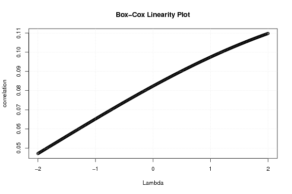
| Title produced by software | Box-Cox Linearity Plot | ||||||||||||||||||||||||||||||||||||||||||||
| Date of computation | Sat, 25 Dec 2010 10:30:27 +0000 | ||||||||||||||||||||||||||||||||||||||||||||
| Cite this page as follows | Statistical Computations at FreeStatistics.org, Office for Research Development and Education, URL https://freestatistics.org/blog/index.php?v=date/2010/Dec/25/t1293272895iq0bbmrg4j7ascx.htm/, Retrieved Sun, 28 Apr 2024 20:41:02 +0000 | ||||||||||||||||||||||||||||||||||||||||||||
| Statistical Computations at FreeStatistics.org, Office for Research Development and Education, URL https://freestatistics.org/blog/index.php?pk=115344, Retrieved Sun, 28 Apr 2024 20:41:02 +0000 | |||||||||||||||||||||||||||||||||||||||||||||
| QR Codes: | |||||||||||||||||||||||||||||||||||||||||||||
|
| |||||||||||||||||||||||||||||||||||||||||||||
| Original text written by user: | |||||||||||||||||||||||||||||||||||||||||||||
| IsPrivate? | No (this computation is public) | ||||||||||||||||||||||||||||||||||||||||||||
| User-defined keywords | |||||||||||||||||||||||||||||||||||||||||||||
| Estimated Impact | 173 | ||||||||||||||||||||||||||||||||||||||||||||
Tree of Dependent Computations | |||||||||||||||||||||||||||||||||||||||||||||
| Family? (F = Feedback message, R = changed R code, M = changed R Module, P = changed Parameters, D = changed Data) | |||||||||||||||||||||||||||||||||||||||||||||
| - [Kendall tau Correlation Matrix] [3/11/2009] [2009-11-02 21:25:00] [b98453cac15ba1066b407e146608df68] - R D [Kendall tau Correlation Matrix] [Kendall tau corre...] [2009-11-12 15:08:30] [54d83950395cfb8ca1091bdb7440f70a] - PD [Kendall tau Correlation Matrix] [Kendall Tau Corre...] [2010-12-25 09:42:33] [1ec36cc0fd92fd0f07d0b885ce2c369b] - RMPD [Box-Cox Linearity Plot] [] [2010-12-25 10:30:27] [d42b17bf3b3c0d56878eb3f5a4351e6d] [Current] | |||||||||||||||||||||||||||||||||||||||||||||
| Feedback Forum | |||||||||||||||||||||||||||||||||||||||||||||
Post a new message | |||||||||||||||||||||||||||||||||||||||||||||
Dataset | |||||||||||||||||||||||||||||||||||||||||||||
| Dataseries X: | |||||||||||||||||||||||||||||||||||||||||||||
493 514 522 490 484 506 501 462 465 454 464 427 460 473 465 422 415 413 420 363 376 380 384 346 389 407 393 346 348 353 364 305 307 312 312 286 324 336 327 302 299 311 315 264 278 278 287 279 324 354 354 360 363 385 412 370 389 395 417 404 | |||||||||||||||||||||||||||||||||||||||||||||
| Dataseries Y: | |||||||||||||||||||||||||||||||||||||||||||||
11 495 13 964 15 751 16 662 16 913 17 017 18 704 18 901 18 123 17 789 17 268 24 042 13 671 15 698 18 150 16 245 18 479 18 479 18 819 18 059 17 004 16 981 16 578 21 604 13 419 14 487 17 349 15 646 17 419 17 358 18 221 19 554 14 386 16 833 18 067 19 662 12 192 15 081 13 698 18 474 13 871 15 669 17 597 15 469 15 374 16 568 11 619 16 780 8 700 8 906 9 612 10 073 10 275 9 921 13 237 9 572 10 425 11 385 9 970 15 456 | |||||||||||||||||||||||||||||||||||||||||||||
Tables (Output of Computation) | |||||||||||||||||||||||||||||||||||||||||||||
| |||||||||||||||||||||||||||||||||||||||||||||
Figures (Output of Computation) | |||||||||||||||||||||||||||||||||||||||||||||
Input Parameters & R Code | |||||||||||||||||||||||||||||||||||||||||||||
| Parameters (Session): | |||||||||||||||||||||||||||||||||||||||||||||
| par1 = Totale werkloze beroepsbevolking ; par2 = CBS ; par3 = Totale werkloze beroepsbevolking ; par4 = 12 ; | |||||||||||||||||||||||||||||||||||||||||||||
| Parameters (R input): | |||||||||||||||||||||||||||||||||||||||||||||
| par1 = pearson ; par2 = ; par3 = ; par4 = ; par5 = ; par6 = ; par7 = ; par8 = ; par9 = ; par10 = ; par11 = ; par12 = ; par13 = ; par14 = ; par15 = ; par16 = ; par17 = ; par18 = ; par19 = ; par20 = ; | |||||||||||||||||||||||||||||||||||||||||||||
| R code (references can be found in the software module): | |||||||||||||||||||||||||||||||||||||||||||||
n <- length(x) | |||||||||||||||||||||||||||||||||||||||||||||