Free Statistics

of Irreproducible Research!

Author's title

Author*The author of this computation has been verified*
R Software Modulerwasp_regression_trees.wasp
Title produced by softwareRecursive Partitioning (Regression Trees)
Date of computationFri, 24 Dec 2010 17:49:39 +0000
Cite this page as followsStatistical Computations at FreeStatistics.org, Office for Research Development and Education, URL https://freestatistics.org/blog/index.php?v=date/2010/Dec/24/t1293212848wou3x5othvb4pqs.htm/, Retrieved Tue, 30 Apr 2024 01:34:40 +0000
Statistical Computations at FreeStatistics.org, Office for Research Development and Education, URL https://freestatistics.org/blog/index.php?pk=115251, Retrieved Tue, 30 Apr 2024 01:34:40 +0000
QR Codes:

Original text written by user:
IsPrivate?No (this computation is public)
User-defined keywords
Estimated Impact154
Family? (F = Feedback message, R = changed R code, M = changed R Module, P = changed Parameters, D = changed Data)
-     [Kendall tau Correlation Matrix] [workshop 3 Q4] [2007-11-29 11:24:56] [74be16979710d4c4e7c6647856088456]
- RMPD    [Recursive Partitioning (Regression Trees)] [workshop 10] [2010-12-24 17:49:39] [36a5183bc8f6439b2481209b0fbe6bda] [Current]
Feedback Forum

Post a new message
Dataseries X:
235.1	9700
280.7	9081
264.6	9084
240.7	9743
201.4	8587
240.8	9731
241.1	9563
223.8	9998
206.1	9437
174.7	10038
203.3	9918
220.5	9252
299.5	9737
347.4	9035
338.3	9133
327.7	9487
351.6	8700
396.6	9627
438.8	8947
395.6	9283
363.5	8829
378.8	9947
357	9628
369	9318
464.8	9605
479.1	8640
431.3	9214
366.5	9567
326.3	8547
355.1	9185
331.6	9470
261.3	9123
249	9278
205.5	10170
235.6	9434
240.9	9655
264.9	9429
253.8	8739
232.3	9552
193.8	9687
177	9019
213.2	9672
207.2	9206
180.6	9069
188.6	9788
175.4	10312
199	10105
179.6	9863
225.8	9656
234	9295
200.2	9946
183.6	9701
178.2	9049
203.2	10190
208.5	9706
191.8	9765
172.8	9893
148	9994
159.4	10433
154.5	10073
213.2	10112
196.4	9266
182.8	9820
176.4	10097
153.6	9115
173.2	10411
171	9678
151.2	10408
161.9	10153
157.2	10368
201.7	10581
236.4	10597
356.1	10680
398.3	9738
403.7	9556


Summary of computational transaction
Raw Inputview raw input (R code)
Raw Outputview raw output of R engine
Computing time3 seconds
R Server'Gwilym Jenkins' @ 72.249.127.135

\begin{tabular}{lllllllll}
\hline
Summary of computational transaction \tabularnewline
Raw Input & view raw input (R code)  \tabularnewline
Raw Output & view raw output of R engine  \tabularnewline
Computing time & 3 seconds \tabularnewline
R Server & 'Gwilym Jenkins' @ 72.249.127.135 \tabularnewline
\hline
\end{tabular}
%Source: https://freestatistics.org/blog/index.php?pk=115251&T=0

[TABLE]
[ROW][C]Summary of computational transaction[/C][/ROW]
[ROW][C]Raw Input[/C][C]view raw input (R code) [/C][/ROW]
[ROW][C]Raw Output[/C][C]view raw output of R engine [/C][/ROW]
[ROW][C]Computing time[/C][C]3 seconds[/C][/ROW]
[ROW][C]R Server[/C][C]'Gwilym Jenkins' @ 72.249.127.135[/C][/ROW]
[/TABLE]
Source: https://freestatistics.org/blog/index.php?pk=115251&T=0

Globally Unique Identifier (entire table): ba.freestatistics.org/blog/index.php?pk=115251&T=0

As an alternative you can also use a QR Code:  

The GUIDs for individual cells are displayed in the table below:

Summary of computational transaction
Raw Inputview raw input (R code)
Raw Outputview raw output of R engine
Computing time3 seconds
R Server'Gwilym Jenkins' @ 72.249.127.135


Model Performance
#Complexitysplitrelative errorCV errorCV S.D.
10.261011.0410.152
20.05410.7390.7720.128
30.02730.6310.8710.15
40.02240.6040.8730.15
50.0150.5820.8560.149

\begin{tabular}{lllllllll}
\hline
Model Performance \tabularnewline
# & Complexity & split & relative error & CV error & CV S.D. \tabularnewline
1 & 0.261 & 0 & 1 & 1.041 & 0.152 \tabularnewline
2 & 0.054 & 1 & 0.739 & 0.772 & 0.128 \tabularnewline
3 & 0.027 & 3 & 0.631 & 0.871 & 0.15 \tabularnewline
4 & 0.022 & 4 & 0.604 & 0.873 & 0.15 \tabularnewline
5 & 0.01 & 5 & 0.582 & 0.856 & 0.149 \tabularnewline
\hline
\end{tabular}
%Source: https://freestatistics.org/blog/index.php?pk=115251&T=1

[TABLE]
[ROW][C]Model Performance[/C][/ROW]
[ROW][C]#[/C][C]Complexity[/C][C]split[/C][C]relative error[/C][C]CV error[/C][C]CV S.D.[/C][/ROW]
[ROW][C]1[/C][C]0.261[/C][C]0[/C][C]1[/C][C]1.041[/C][C]0.152[/C][/ROW]
[ROW][C]2[/C][C]0.054[/C][C]1[/C][C]0.739[/C][C]0.772[/C][C]0.128[/C][/ROW]
[ROW][C]3[/C][C]0.027[/C][C]3[/C][C]0.631[/C][C]0.871[/C][C]0.15[/C][/ROW]
[ROW][C]4[/C][C]0.022[/C][C]4[/C][C]0.604[/C][C]0.873[/C][C]0.15[/C][/ROW]
[ROW][C]5[/C][C]0.01[/C][C]5[/C][C]0.582[/C][C]0.856[/C][C]0.149[/C][/ROW]
[/TABLE]
Source: https://freestatistics.org/blog/index.php?pk=115251&T=1

Globally Unique Identifier (entire table): ba.freestatistics.org/blog/index.php?pk=115251&T=1

As an alternative you can also use a QR Code:  

The GUIDs for individual cells are displayed in the table below:

Model Performance
#Complexitysplitrelative errorCV errorCV S.D.
10.261011.0410.152
20.05410.7390.7720.128
30.02730.6310.8710.15
40.02240.6040.8730.15
50.0150.5820.8560.149


Parameters (Session):
par1 = kendall ;
Parameters (R input):
par1 = 1 ; par2 = No ;
R code (references can be found in the software module):
library(rpart)
library(partykit)
par1 <- as.numeric(par1)
autoprune <- function ( tree, method='Minimum CV'){
xerr <- tree$cptable[,'xerror']
cpmin.id <- which.min(xerr)
if (method == 'Minimum CV Error plus 1 SD'){
xstd <- tree$cptable[,'xstd']
errt <- xerr[cpmin.id] + xstd[cpmin.id]
cpSE1.min <- which.min( errt < xerr )
mycp <- (tree$cptable[,'CP'])[cpSE1.min]
}
if (method == 'Minimum CV') {
mycp <- (tree$cptable[,'CP'])[cpmin.id]
}
return (mycp)
}
conf.multi.mat <- function(true, new)
{
if ( all( is.na(match( levels(true),levels(new) ) )) )
stop ( 'conflict of vector levels')
multi.t <- list()
for (mylev in levels(true) ) {
true.tmp <- true
new.tmp <- new
left.lev <- levels (true.tmp)[- match(mylev,levels(true) ) ]
levels(true.tmp) <- list ( mylev = mylev, all = left.lev )
levels(new.tmp) <- list ( mylev = mylev, all = left.lev )
curr.t <- conf.mat ( true.tmp , new.tmp )
multi.t[[mylev]] <- curr.t
multi.t[[mylev]]$precision <-
round( curr.t$conf[1,1] / sum( curr.t$conf[1,] ), 2 )
}
return (multi.t)
}
x <- t(y)
k <- length(x[1,])
n <- length(x[,1])
x1 <- cbind(x[,par1], x[,1:k!=par1])
mycolnames <- c(colnames(x)[par1], colnames(x)[1:k!=par1])
colnames(x1) <- mycolnames #colnames(x)[par1]
m <- rpart(as.data.frame(x1))
par2
if (par2 != 'No') {
mincp <- autoprune(m,method=par2)
print(mincp)
m <- prune(m,cp=mincp)
}
m$cptable
bitmap(file='test1.png')
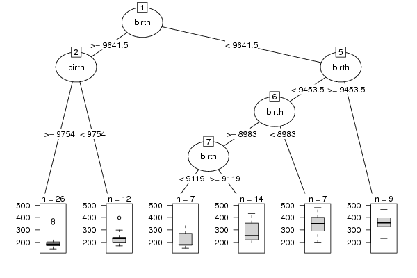
plot(as.party(m),tp_args=list(id=FALSE))
dev.off()
bitmap(file='test2.png')
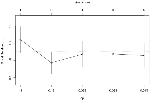
plotcp(m)
dev.off()
cbind(y=m$y,pred=predict(m),res=residuals(m))
myr <- residuals(m)
myp <- predict(m)
bitmap(file='test4.png')
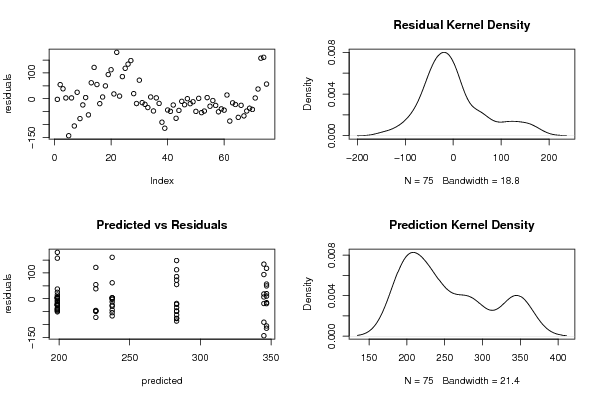
op <- par(mfrow=c(2,2))
plot(myr,ylab='residuals')
plot(density(myr),main='Residual Kernel Density')
plot(myp,myr,xlab='predicted',ylab='residuals',main='Predicted vs Residuals')
plot(density(myp),main='Prediction Kernel Density')
par(op)
dev.off()
load(file='createtable')
a<-table.start()
a<-table.row.start(a)
a<-table.element(a,'Model Performance',6,TRUE)
a<-table.row.end(a)
a<-table.row.start(a)
a<-table.element(a,'#',header=TRUE)
a<-table.element(a,'Complexity',header=TRUE)
a<-table.element(a,'split',header=TRUE)
a<-table.element(a,'relative error',header=TRUE)
a<-table.element(a,'CV error',header=TRUE)
a<-table.element(a,'CV S.D.',header=TRUE)
a<-table.row.end(a)
for (i in 1:length(m$cptable[,1])) {
a<-table.row.start(a)
a<-table.element(a,i,header=TRUE)
a<-table.element(a,round(m$cptable[i,'CP'],3))
a<-table.element(a,m$cptable[i,'nsplit'])
a<-table.element(a,round(m$cptable[i,'rel error'],3))
a<-table.element(a,round(m$cptable[i,'xerror'],3))
a<-table.element(a,round(m$cptable[i,'xstd'],3))
a<-table.row.end(a)
}
a<-table.end(a)
table.save(a,file='mytable.tab')