Repository of Reproducible Computations

Free Statistics

of Irreproducible Research!

Author's title

Author

*The author of this computation has been verified*

R Software Module

rwasp_autocorrelation.wasp

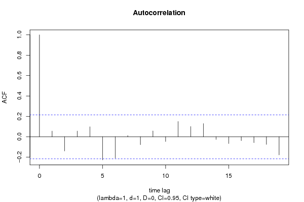
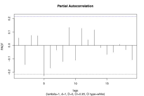
Title produced by software

(Partial) Autocorrelation Function

Date of computation

Fri, 24 Dec 2010 16:55:11 +0000

Cite this page as follows

Statistical Computations at FreeStatistics.org, Office for Research Development and Education, URL https://freestatistics.org/blog/index.php?v=date/2010/Dec/24/t1293209592f74frtxxjflenri.htm/, Retrieved Tue, 30 Apr 2024 03:35:49 +0000

Statistical Computations at FreeStatistics.org, Office for Research Development and Education, URL https://freestatistics.org/blog/index.php?pk=115201, Retrieved Tue, 30 Apr 2024 03:35:49 +0000

QR Codes:

Paste this QR Code to cite your computation.

Original text written by user:

IsPrivate?

No (this computation is public)

User-defined keywords

Estimated Impact

126

Family? (F = Feedback message, R = changed R code, M = changed R Module, P = changed Parameters, D = changed Data)

-     [Univariate Data Series] [data set] [2008-12-01 19:54:57] [b98453cac15ba1066b407e146608df68]
- RMP   [(Partial) Autocorrelation Function] [Unemployment] [2010-11-29 09:05:21] [b98453cac15ba1066b407e146608df68]
- R PD    [(Partial) Autocorrelation Function] [ACF van de goudpr...] [2010-12-24 16:13:00] [96348ef82925ade81ab3c243141d80f1]
-    D      [(Partial) Autocorrelation Function] [autocorrelatiefun...] [2010-12-24 16:50:22] [96348ef82925ade81ab3c243141d80f1]
-    D          [(Partial) Autocorrelation Function] [autocorrelatiefun...] [2010-12-24 16:55:11] [03bcd8c83ef1a42b4029a16ba47a4880] [Current]
-   PD            [(Partial) Autocorrelation Function] [ACF goudprijzen m...] [2010-12-28 18:54:34] [30b3e197115d238a51c18bcedc33a6a5] 

Feedback Forum

Post a new message

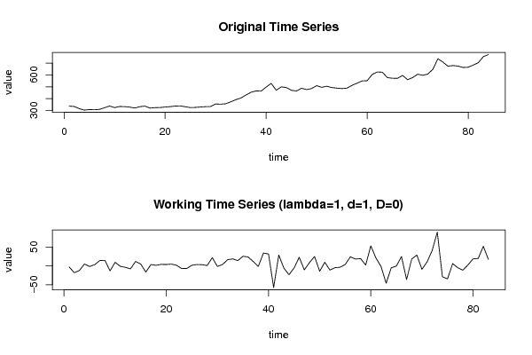
Dataseries X:

Download CSV

Histogram

Boxplots

Summary of computational transaction
Raw Input	view raw input (R code)
Raw Output	view raw output of R engine
Computing time	1 seconds
R Server	'RServer@AstonUniversity' @ vre.aston.ac.uk

\begin{tabular}{lllllllll}
\hline
Summary of computational transaction \tabularnewline
Raw Input & view raw input (R code)  \tabularnewline
Raw Output & view raw output of R engine  \tabularnewline
Computing time & 1 seconds \tabularnewline
R Server & 'RServer@AstonUniversity' @ vre.aston.ac.uk \tabularnewline
\hline
\end{tabular}
%Source: https://freestatistics.org/blog/index.php?pk=115201&T=0

[TABLE]
[ROW][C]Summary of computational transaction[/C][/ROW]
[ROW][C]Raw Input[/C][C]view raw input (R code) [/C][/ROW]
[ROW][C]Raw Output[/C][C]view raw output of R engine [/C][/ROW]
[ROW][C]Computing time[/C][C]1 seconds[/C][/ROW]
[ROW][C]R Server[/C][C]'RServer@AstonUniversity' @ vre.aston.ac.uk[/C][/ROW]
[/TABLE]
Source: https://freestatistics.org/blog/index.php?pk=115201&T=0

Globally Unique Identifier (entire table): ba.freestatistics.org/blog/index.php?pk=115201&T=0

As an alternative you can also use a QR Code:

The GUIDs for individual cells are displayed in the table below:

Summary of computational transaction
Raw Input	view raw input (R code)
Raw Output	view raw output of R engine
Computing time	1 seconds
R Server	'RServer@AstonUniversity' @ vre.aston.ac.uk

Autocorrelation Function
Time lag k	ACF(k)	T-STAT	P-value
1	0.055538	0.506	0.307108
2	-0.139747	-1.2732	0.103259
3	0.056073	0.5109	0.305405
4	0.098791	0.9	0.185355
5	-0.227002	-2.0681	0.020873
6	-0.209149	-1.9054	0.030093
7	0.011686	0.1065	0.457737
8	-0.077806	-0.7088	0.240204
9	0.057343	0.5224	0.301385
10	-0.046806	-0.4264	0.335451
11	0.15017	1.3681	0.087485
12	0.100925	0.9195	0.180256
13	0.129132	1.1764	0.12139
14	-0.026284	-0.2395	0.40567
15	-0.06657	-0.6065	0.272925
16	-0.038429	-0.3501	0.363574
17	-0.057799	-0.5266	0.299946
18	-0.075463	-0.6875	0.246842
19	-0.178095	-1.6225	0.054242

\begin{tabular}{lllllllll}
\hline
Autocorrelation Function \tabularnewline
Time lag k & ACF(k) & T-STAT & P-value \tabularnewline
1 & 0.055538 & 0.506 & 0.307108 \tabularnewline
2 & -0.139747 & -1.2732 & 0.103259 \tabularnewline
3 & 0.056073 & 0.5109 & 0.305405 \tabularnewline
4 & 0.098791 & 0.9 & 0.185355 \tabularnewline
5 & -0.227002 & -2.0681 & 0.020873 \tabularnewline
6 & -0.209149 & -1.9054 & 0.030093 \tabularnewline
7 & 0.011686 & 0.1065 & 0.457737 \tabularnewline
8 & -0.077806 & -0.7088 & 0.240204 \tabularnewline
9 & 0.057343 & 0.5224 & 0.301385 \tabularnewline
10 & -0.046806 & -0.4264 & 0.335451 \tabularnewline
11 & 0.15017 & 1.3681 & 0.087485 \tabularnewline
12 & 0.100925 & 0.9195 & 0.180256 \tabularnewline
13 & 0.129132 & 1.1764 & 0.12139 \tabularnewline
14 & -0.026284 & -0.2395 & 0.40567 \tabularnewline
15 & -0.06657 & -0.6065 & 0.272925 \tabularnewline
16 & -0.038429 & -0.3501 & 0.363574 \tabularnewline
17 & -0.057799 & -0.5266 & 0.299946 \tabularnewline
18 & -0.075463 & -0.6875 & 0.246842 \tabularnewline
19 & -0.178095 & -1.6225 & 0.054242 \tabularnewline
\hline
\end{tabular}
%Source: https://freestatistics.org/blog/index.php?pk=115201&T=1

[TABLE]
[ROW][C]Autocorrelation Function[/C][/ROW]
[ROW][C]Time lag k[/C][C]ACF(k)[/C][C]T-STAT[/C][C]P-value[/C][/ROW]
[ROW][C]1[/C][C]0.055538[/C][C]0.506[/C][C]0.307108[/C][/ROW]
[ROW][C]2[/C][C]-0.139747[/C][C]-1.2732[/C][C]0.103259[/C][/ROW]
[ROW][C]3[/C][C]0.056073[/C][C]0.5109[/C][C]0.305405[/C][/ROW]
[ROW][C]4[/C][C]0.098791[/C][C]0.9[/C][C]0.185355[/C][/ROW]
[ROW][C]5[/C][C]-0.227002[/C][C]-2.0681[/C][C]0.020873[/C][/ROW]
[ROW][C]6[/C][C]-0.209149[/C][C]-1.9054[/C][C]0.030093[/C][/ROW]
[ROW][C]7[/C][C]0.011686[/C][C]0.1065[/C][C]0.457737[/C][/ROW]
[ROW][C]8[/C][C]-0.077806[/C][C]-0.7088[/C][C]0.240204[/C][/ROW]
[ROW][C]9[/C][C]0.057343[/C][C]0.5224[/C][C]0.301385[/C][/ROW]
[ROW][C]10[/C][C]-0.046806[/C][C]-0.4264[/C][C]0.335451[/C][/ROW]
[ROW][C]11[/C][C]0.15017[/C][C]1.3681[/C][C]0.087485[/C][/ROW]
[ROW][C]12[/C][C]0.100925[/C][C]0.9195[/C][C]0.180256[/C][/ROW]
[ROW][C]13[/C][C]0.129132[/C][C]1.1764[/C][C]0.12139[/C][/ROW]
[ROW][C]14[/C][C]-0.026284[/C][C]-0.2395[/C][C]0.40567[/C][/ROW]
[ROW][C]15[/C][C]-0.06657[/C][C]-0.6065[/C][C]0.272925[/C][/ROW]
[ROW][C]16[/C][C]-0.038429[/C][C]-0.3501[/C][C]0.363574[/C][/ROW]
[ROW][C]17[/C][C]-0.057799[/C][C]-0.5266[/C][C]0.299946[/C][/ROW]
[ROW][C]18[/C][C]-0.075463[/C][C]-0.6875[/C][C]0.246842[/C][/ROW]
[ROW][C]19[/C][C]-0.178095[/C][C]-1.6225[/C][C]0.054242[/C][/ROW]
[/TABLE]
Source: https://freestatistics.org/blog/index.php?pk=115201&T=1

Globally Unique Identifier (entire table): ba.freestatistics.org/blog/index.php?pk=115201&T=1

As an alternative you can also use a QR Code:

The GUIDs for individual cells are displayed in the table below:

Autocorrelation Function
Time lag k	ACF(k)	T-STAT	P-value
1	0.055538	0.506	0.307108
2	-0.139747	-1.2732	0.103259
3	0.056073	0.5109	0.305405
4	0.098791	0.9	0.185355
5	-0.227002	-2.0681	0.020873
6	-0.209149	-1.9054	0.030093
7	0.011686	0.1065	0.457737
8	-0.077806	-0.7088	0.240204
9	0.057343	0.5224	0.301385
10	-0.046806	-0.4264	0.335451
11	0.15017	1.3681	0.087485
12	0.100925	0.9195	0.180256
13	0.129132	1.1764	0.12139
14	-0.026284	-0.2395	0.40567
15	-0.06657	-0.6065	0.272925
16	-0.038429	-0.3501	0.363574
17	-0.057799	-0.5266	0.299946
18	-0.075463	-0.6875	0.246842
19	-0.178095	-1.6225	0.054242

Partial Autocorrelation Function
Time lag k	PACF(k)	T-STAT	P-value
1	0.055538	0.506	0.307108
2	-0.143273	-1.3053	0.097702
3	0.074662	0.6802	0.249135
4	0.071884	0.6549	0.257174
5	-0.228161	-2.0786	0.020369
6	-0.169282	-1.5422	0.06341
7	-0.035311	-0.3217	0.374246
8	-0.121129	-1.1035	0.136491
9	0.133728	1.2183	0.113277
10	-0.11057	-1.0073	0.15835
11	0.126558	1.153	0.126111
12	0.042035	0.383	0.351365
13	0.115751	1.0545	0.147348
14	-0.01767	-0.161	0.436248
15	-0.067748	-0.6172	0.269392
16	-0.0514	-0.4683	0.320407
17	0.009012	0.0821	0.467382
18	-0.032328	-0.2945	0.384548
19	-0.108129	-0.9851	0.163719

\begin{tabular}{lllllllll}
\hline
Partial Autocorrelation Function \tabularnewline
Time lag k & PACF(k) & T-STAT & P-value \tabularnewline
1 & 0.055538 & 0.506 & 0.307108 \tabularnewline
2 & -0.143273 & -1.3053 & 0.097702 \tabularnewline
3 & 0.074662 & 0.6802 & 0.249135 \tabularnewline
4 & 0.071884 & 0.6549 & 0.257174 \tabularnewline
5 & -0.228161 & -2.0786 & 0.020369 \tabularnewline
6 & -0.169282 & -1.5422 & 0.06341 \tabularnewline
7 & -0.035311 & -0.3217 & 0.374246 \tabularnewline
8 & -0.121129 & -1.1035 & 0.136491 \tabularnewline
9 & 0.133728 & 1.2183 & 0.113277 \tabularnewline
10 & -0.11057 & -1.0073 & 0.15835 \tabularnewline
11 & 0.126558 & 1.153 & 0.126111 \tabularnewline
12 & 0.042035 & 0.383 & 0.351365 \tabularnewline
13 & 0.115751 & 1.0545 & 0.147348 \tabularnewline
14 & -0.01767 & -0.161 & 0.436248 \tabularnewline
15 & -0.067748 & -0.6172 & 0.269392 \tabularnewline
16 & -0.0514 & -0.4683 & 0.320407 \tabularnewline
17 & 0.009012 & 0.0821 & 0.467382 \tabularnewline
18 & -0.032328 & -0.2945 & 0.384548 \tabularnewline
19 & -0.108129 & -0.9851 & 0.163719 \tabularnewline
\hline
\end{tabular}
%Source: https://freestatistics.org/blog/index.php?pk=115201&T=2

[TABLE]
[ROW][C]Partial Autocorrelation Function[/C][/ROW]
[ROW][C]Time lag k[/C][C]PACF(k)[/C][C]T-STAT[/C][C]P-value[/C][/ROW]
[ROW][C]1[/C][C]0.055538[/C][C]0.506[/C][C]0.307108[/C][/ROW]
[ROW][C]2[/C][C]-0.143273[/C][C]-1.3053[/C][C]0.097702[/C][/ROW]
[ROW][C]3[/C][C]0.074662[/C][C]0.6802[/C][C]0.249135[/C][/ROW]
[ROW][C]4[/C][C]0.071884[/C][C]0.6549[/C][C]0.257174[/C][/ROW]
[ROW][C]5[/C][C]-0.228161[/C][C]-2.0786[/C][C]0.020369[/C][/ROW]
[ROW][C]6[/C][C]-0.169282[/C][C]-1.5422[/C][C]0.06341[/C][/ROW]
[ROW][C]7[/C][C]-0.035311[/C][C]-0.3217[/C][C]0.374246[/C][/ROW]
[ROW][C]8[/C][C]-0.121129[/C][C]-1.1035[/C][C]0.136491[/C][/ROW]
[ROW][C]9[/C][C]0.133728[/C][C]1.2183[/C][C]0.113277[/C][/ROW]
[ROW][C]10[/C][C]-0.11057[/C][C]-1.0073[/C][C]0.15835[/C][/ROW]
[ROW][C]11[/C][C]0.126558[/C][C]1.153[/C][C]0.126111[/C][/ROW]
[ROW][C]12[/C][C]0.042035[/C][C]0.383[/C][C]0.351365[/C][/ROW]
[ROW][C]13[/C][C]0.115751[/C][C]1.0545[/C][C]0.147348[/C][/ROW]
[ROW][C]14[/C][C]-0.01767[/C][C]-0.161[/C][C]0.436248[/C][/ROW]
[ROW][C]15[/C][C]-0.067748[/C][C]-0.6172[/C][C]0.269392[/C][/ROW]
[ROW][C]16[/C][C]-0.0514[/C][C]-0.4683[/C][C]0.320407[/C][/ROW]
[ROW][C]17[/C][C]0.009012[/C][C]0.0821[/C][C]0.467382[/C][/ROW]
[ROW][C]18[/C][C]-0.032328[/C][C]-0.2945[/C][C]0.384548[/C][/ROW]
[ROW][C]19[/C][C]-0.108129[/C][C]-0.9851[/C][C]0.163719[/C][/ROW]
[/TABLE]
Source: https://freestatistics.org/blog/index.php?pk=115201&T=2

Globally Unique Identifier (entire table): ba.freestatistics.org/blog/index.php?pk=115201&T=2

As an alternative you can also use a QR Code:

The GUIDs for individual cells are displayed in the table below:

Partial Autocorrelation Function
Time lag k	PACF(k)	T-STAT	P-value
1	0.055538	0.506	0.307108
2	-0.143273	-1.3053	0.097702
3	0.074662	0.6802	0.249135
4	0.071884	0.6549	0.257174
5	-0.228161	-2.0786	0.020369
6	-0.169282	-1.5422	0.06341
7	-0.035311	-0.3217	0.374246
8	-0.121129	-1.1035	0.136491
9	0.133728	1.2183	0.113277
10	-0.11057	-1.0073	0.15835
11	0.126558	1.153	0.126111
12	0.042035	0.383	0.351365
13	0.115751	1.0545	0.147348
14	-0.01767	-0.161	0.436248
15	-0.067748	-0.6172	0.269392
16	-0.0514	-0.4683	0.320407
17	0.009012	0.0821	0.467382
18	-0.032328	-0.2945	0.384548
19	-0.108129	-0.9851	0.163719

Figure 1

PNG link

Postscript link

PDF link

Figure 2

PNG link

Postscript link

PDF link

Figure 3

PNG link

Postscript link

PDF link

Parameters (Session):

par1 = 12 ;

Parameters (R input):

par1 = Default ; par2 = 1 ; par3 = 1 ; par4 = 0 ; par5 = 12 ; par6 = White Noise ; par7 = 0.95 ; par8 = ;

R code (references can be found in the software module):

if (par1 == 'Default') {
par1 = 10*log10(length(x))
} else {
par1 <- as.numeric(par1)
}
par2 <- as.numeric(par2)
par3 <- as.numeric(par3)
par4 <- as.numeric(par4)
par5 <- as.numeric(par5)
if (par6 == 'White Noise') par6 <- 'white' else par6 <- 'ma'
par7 <- as.numeric(par7)
if (par8 != '') par8 <- as.numeric(par8)
ox <- x
if (par8 == '') {
if (par2 == 0) {
x <- log(x)
} else {
x <- (x ^ par2 - 1) / par2
}
} else {
x <- log(x,base=par8)
}
if (par3 > 0) x <- diff(x,lag=1,difference=par3)
if (par4 > 0) x <- diff(x,lag=par5,difference=par4)
bitmap(file='picts.png')
op <- par(mfrow=c(2,1))
plot(ox,type='l',main='Original Time Series',xlab='time',ylab='value')
if (par8=='') {
mytitle <- paste('Working Time Series (lambda=',par2,', d=',par3,', D=',par4,')',sep='')
mysub <- paste('(lambda=',par2,', d=',par3,', D=',par4,', CI=', par7, ', CI type=',par6,')',sep='')
} else {
mytitle <- paste('Working Time Series (base=',par8,', d=',par3,', D=',par4,')',sep='')
mysub <- paste('(base=',par8,', d=',par3,', D=',par4,', CI=', par7, ', CI type=',par6,')',sep='')
}
plot(x,type='l', main=mytitle,xlab='time',ylab='value')
par(op)
dev.off()
bitmap(file='pic1.png')
racf <- acf(x, par1, main='Autocorrelation', xlab='time lag', ylab='ACF', ci.type=par6, ci=par7, sub=mysub)
dev.off()
bitmap(file='pic2.png')
rpacf <- pacf(x,par1,main='Partial Autocorrelation',xlab='lags',ylab='PACF',sub=mysub)
dev.off()
(myacf <- c(racf$acf))
(mypacf <- c(rpacf$acf))
lengthx <- length(x)
sqrtn <- sqrt(lengthx)
load(file='createtable')
a<-table.start()
a<-table.row.start(a)
a<-table.element(a,'Autocorrelation Function',4,TRUE)
a<-table.row.end(a)
a<-table.row.start(a)
a<-table.element(a,'Time lag k',header=TRUE)
a<-table.element(a,hyperlink('basics.htm','ACF(k)','click here for more information about the Autocorrelation Function'),header=TRUE)
a<-table.element(a,'T-STAT',header=TRUE)
a<-table.element(a,'P-value',header=TRUE)
a<-table.row.end(a)
for (i in 2:(par1+1)) {
a<-table.row.start(a)
a<-table.element(a,i-1,header=TRUE)
a<-table.element(a,round(myacf[i],6))
mytstat <- myacf[i]*sqrtn
a<-table.element(a,round(mytstat,4))
a<-table.element(a,round(1-pt(abs(mytstat),lengthx),6))
a<-table.row.end(a)
}
a<-table.end(a)
table.save(a,file='mytable.tab')
a<-table.start()
a<-table.row.start(a)
a<-table.element(a,'Partial Autocorrelation Function',4,TRUE)
a<-table.row.end(a)
a<-table.row.start(a)
a<-table.element(a,'Time lag k',header=TRUE)
a<-table.element(a,hyperlink('basics.htm','PACF(k)','click here for more information about the Partial Autocorrelation Function'),header=TRUE)
a<-table.element(a,'T-STAT',header=TRUE)
a<-table.element(a,'P-value',header=TRUE)
a<-table.row.end(a)
for (i in 1:par1) {
a<-table.row.start(a)
a<-table.element(a,i,header=TRUE)
a<-table.element(a,round(mypacf[i],6))
mytstat <- mypacf[i]*sqrtn
a<-table.element(a,round(mytstat,4))
a<-table.element(a,round(1-pt(abs(mytstat),lengthx),6))
a<-table.row.end(a)
}
a<-table.end(a)
table.save(a,file='mytable1.tab')

Free Statistics

Description of Statistical Computation

Tree of Dependent Computations

Dataset

Tables (Output of Computation)

Figures (Output of Computation)

Input Parameters & R Code