Repository of Reproducible Computations

Free Statistics

of Irreproducible Research!

Author's title

Author

*The author of this computation has been verified*

R Software Module

rwasp_autocorrelation.wasp

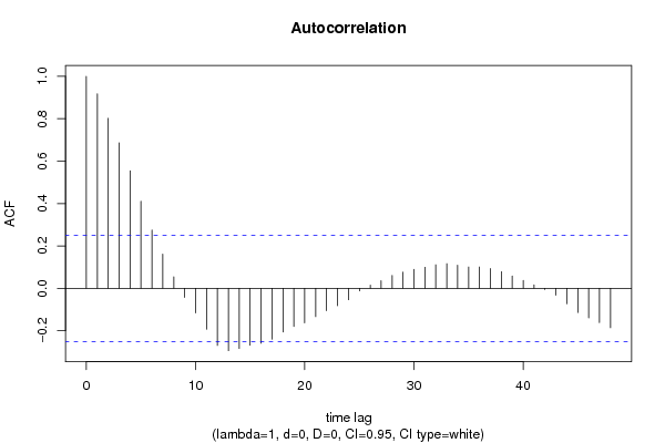
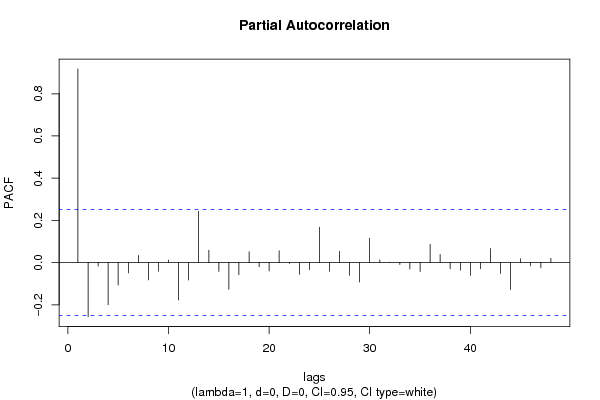
Title produced by software

(Partial) Autocorrelation Function

Date of computation

Fri, 24 Dec 2010 16:52:10 +0000

Cite this page as follows

Statistical Computations at FreeStatistics.org, Office for Research Development and Education, URL https://freestatistics.org/blog/index.php?v=date/2010/Dec/24/t1293209528cdf9l4v3h6aa79t.htm/, Retrieved Tue, 30 Apr 2024 02:33:02 +0000

Statistical Computations at FreeStatistics.org, Office for Research Development and Education, URL https://freestatistics.org/blog/index.php?pk=115199, Retrieved Tue, 30 Apr 2024 02:33:02 +0000

QR Codes:

Paste this QR Code to cite your computation.

Original text written by user:

IsPrivate?

No (this computation is public)

User-defined keywords

Estimated Impact

123

Family? (F = Feedback message, R = changed R code, M = changed R Module, P = changed Parameters, D = changed Data)

-       [(Partial) Autocorrelation Function] [ACF] [2010-12-24 16:52:10] [fd751bc40fbbb4c72222c10190589d42] [Current]
-   PD    [(Partial) Autocorrelation Function] [ACF2] [2010-12-25 08:44:43] [6a528ed37664d761abf4790b0717b23b] 
- RMPD    [Spectral Analysis] [SA] [2010-12-25 09:12:40] [6a528ed37664d761abf4790b0717b23b] 
-   P       [Spectral Analysis] [SA2] [2010-12-25 14:27:23] [6a528ed37664d761abf4790b0717b23b] 
- RMP       [Variance Reduction Matrix] [VRM] [2010-12-25 14:32:01] [6a528ed37664d761abf4790b0717b23b] 
- RMPD    [Box-Cox Normality Plot] [BCT] [2010-12-25 10:02:59] [6a528ed37664d761abf4790b0717b23b] 

Feedback Forum

Post a new message

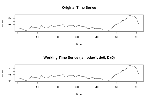
Dataseries X:

Download CSV

Histogram

Boxplots

1,8
1,7
1,4
1,2
1
1,7
2,4
2
2,1
2
1,8
2,7
2,3
1,9
2
2,3
2,8
2,4
2,3
2,7
2,7
2,9
3
2,2
2,3
2,8
2,8
2,8
2,2
2,6
2,8
2,5
2,4
2,3
1,9
1,7
2
2,1
1,7
1,8
1,8
1,8
1,3
1,3
1,3
1,2
1,4
2,2
2,9
3,1
3,5
3,6
4,4
4,1
5,1
5,8
5,9
5,4
5,5
4,8
3,2

Summary of computational transaction
Raw Input	view raw input (R code)
Raw Output	view raw output of R engine
Computing time	2 seconds
R Server	'Sir Ronald Aylmer Fisher' @ 193.190.124.24

\begin{tabular}{lllllllll}
\hline
Summary of computational transaction \tabularnewline
Raw Input & view raw input (R code)  \tabularnewline
Raw Output & view raw output of R engine  \tabularnewline
Computing time & 2 seconds \tabularnewline
R Server & 'Sir Ronald Aylmer Fisher' @ 193.190.124.24 \tabularnewline
\hline
\end{tabular}
%Source: https://freestatistics.org/blog/index.php?pk=115199&T=0

[TABLE]
[ROW][C]Summary of computational transaction[/C][/ROW]
[ROW][C]Raw Input[/C][C]view raw input (R code) [/C][/ROW]
[ROW][C]Raw Output[/C][C]view raw output of R engine [/C][/ROW]
[ROW][C]Computing time[/C][C]2 seconds[/C][/ROW]
[ROW][C]R Server[/C][C]'Sir Ronald Aylmer Fisher' @ 193.190.124.24[/C][/ROW]
[/TABLE]
Source: https://freestatistics.org/blog/index.php?pk=115199&T=0

Globally Unique Identifier (entire table): ba.freestatistics.org/blog/index.php?pk=115199&T=0

As an alternative you can also use a QR Code:

The GUIDs for individual cells are displayed in the table below:

Summary of computational transaction
Raw Input	view raw input (R code)
Raw Output	view raw output of R engine
Computing time	2 seconds
R Server	'Sir Ronald Aylmer Fisher' @ 193.190.124.24

Autocorrelation Function
Time lag k	ACF(k)	T-STAT	P-value
1	0.917746	7.1678	0
2	0.801812	6.2623	0
3	0.686775	5.3639	1e-06
4	0.553946	4.3265	2.9e-05
5	0.411153	3.2112	0.001055
6	0.275331	2.1504	0.017748
7	0.160907	1.2567	0.106822
8	0.054346	0.4245	0.336365
9	-0.042759	-0.334	0.369777
10	-0.116329	-0.9086	0.183579
11	-0.192774	-1.5056	0.068664
12	-0.269563	-2.1054	0.019693
13	-0.294388	-2.2992	0.012465
14	-0.284022	-2.2183	0.015134
15	-0.269114	-2.1018	0.019852
16	-0.258995	-2.0228	0.023741
17	-0.240681	-1.8798	0.032458
18	-0.206391	-1.612	0.056066
19	-0.180396	-1.4089	0.081965
20	-0.162652	-1.2704	0.104392
21	-0.133781	-1.0449	0.150105
22	-0.105805	-0.8264	0.205909
23	-0.08162	-0.6375	0.263101
24	-0.054054	-0.4222	0.337191
25	-0.012181	-0.0951	0.462258
26	0.014856	0.116	0.454005
27	0.035862	0.2801	0.390178
28	0.060945	0.476	0.31789
29	0.076468	0.5972	0.27628
30	0.089324	0.6976	0.244026
31	0.099022	0.7734	0.22114
32	0.111022	0.8671	0.194641
33	0.116152	0.9072	0.183942
34	0.109077	0.8519	0.198796
35	0.10037	0.7839	0.218062
36	0.100507	0.785	0.21775
37	0.093226	0.7281	0.234665
38	0.078363	0.612	0.271395
39	0.058407	0.4562	0.324943
40	0.036861	0.2879	0.387201
41	0.016456	0.1285	0.449077
42	-0.005538	-0.0433	0.48282
43	-0.031999	-0.2499	0.401745
44	-0.073152	-0.5713	0.284935
45	-0.114019	-0.8905	0.188344
46	-0.140093	-1.0942	0.139094
47	-0.161744	-1.2633	0.105651
48	-0.18586	-1.4516	0.075867

\begin{tabular}{lllllllll}
\hline
Autocorrelation Function \tabularnewline
Time lag k & ACF(k) & T-STAT & P-value \tabularnewline
1 & 0.917746 & 7.1678 & 0 \tabularnewline
2 & 0.801812 & 6.2623 & 0 \tabularnewline
3 & 0.686775 & 5.3639 & 1e-06 \tabularnewline
4 & 0.553946 & 4.3265 & 2.9e-05 \tabularnewline
5 & 0.411153 & 3.2112 & 0.001055 \tabularnewline
6 & 0.275331 & 2.1504 & 0.017748 \tabularnewline
7 & 0.160907 & 1.2567 & 0.106822 \tabularnewline
8 & 0.054346 & 0.4245 & 0.336365 \tabularnewline
9 & -0.042759 & -0.334 & 0.369777 \tabularnewline
10 & -0.116329 & -0.9086 & 0.183579 \tabularnewline
11 & -0.192774 & -1.5056 & 0.068664 \tabularnewline
12 & -0.269563 & -2.1054 & 0.019693 \tabularnewline
13 & -0.294388 & -2.2992 & 0.012465 \tabularnewline
14 & -0.284022 & -2.2183 & 0.015134 \tabularnewline
15 & -0.269114 & -2.1018 & 0.019852 \tabularnewline
16 & -0.258995 & -2.0228 & 0.023741 \tabularnewline
17 & -0.240681 & -1.8798 & 0.032458 \tabularnewline
18 & -0.206391 & -1.612 & 0.056066 \tabularnewline
19 & -0.180396 & -1.4089 & 0.081965 \tabularnewline
20 & -0.162652 & -1.2704 & 0.104392 \tabularnewline
21 & -0.133781 & -1.0449 & 0.150105 \tabularnewline
22 & -0.105805 & -0.8264 & 0.205909 \tabularnewline
23 & -0.08162 & -0.6375 & 0.263101 \tabularnewline
24 & -0.054054 & -0.4222 & 0.337191 \tabularnewline
25 & -0.012181 & -0.0951 & 0.462258 \tabularnewline
26 & 0.014856 & 0.116 & 0.454005 \tabularnewline
27 & 0.035862 & 0.2801 & 0.390178 \tabularnewline
28 & 0.060945 & 0.476 & 0.31789 \tabularnewline
29 & 0.076468 & 0.5972 & 0.27628 \tabularnewline
30 & 0.089324 & 0.6976 & 0.244026 \tabularnewline
31 & 0.099022 & 0.7734 & 0.22114 \tabularnewline
32 & 0.111022 & 0.8671 & 0.194641 \tabularnewline
33 & 0.116152 & 0.9072 & 0.183942 \tabularnewline
34 & 0.109077 & 0.8519 & 0.198796 \tabularnewline
35 & 0.10037 & 0.7839 & 0.218062 \tabularnewline
36 & 0.100507 & 0.785 & 0.21775 \tabularnewline
37 & 0.093226 & 0.7281 & 0.234665 \tabularnewline
38 & 0.078363 & 0.612 & 0.271395 \tabularnewline
39 & 0.058407 & 0.4562 & 0.324943 \tabularnewline
40 & 0.036861 & 0.2879 & 0.387201 \tabularnewline
41 & 0.016456 & 0.1285 & 0.449077 \tabularnewline
42 & -0.005538 & -0.0433 & 0.48282 \tabularnewline
43 & -0.031999 & -0.2499 & 0.401745 \tabularnewline
44 & -0.073152 & -0.5713 & 0.284935 \tabularnewline
45 & -0.114019 & -0.8905 & 0.188344 \tabularnewline
46 & -0.140093 & -1.0942 & 0.139094 \tabularnewline
47 & -0.161744 & -1.2633 & 0.105651 \tabularnewline
48 & -0.18586 & -1.4516 & 0.075867 \tabularnewline
\hline
\end{tabular}
%Source: https://freestatistics.org/blog/index.php?pk=115199&T=1

[TABLE]
[ROW][C]Autocorrelation Function[/C][/ROW]
[ROW][C]Time lag k[/C][C]ACF(k)[/C][C]T-STAT[/C][C]P-value[/C][/ROW]
[ROW][C]1[/C][C]0.917746[/C][C]7.1678[/C][C]0[/C][/ROW]
[ROW][C]2[/C][C]0.801812[/C][C]6.2623[/C][C]0[/C][/ROW]
[ROW][C]3[/C][C]0.686775[/C][C]5.3639[/C][C]1e-06[/C][/ROW]
[ROW][C]4[/C][C]0.553946[/C][C]4.3265[/C][C]2.9e-05[/C][/ROW]
[ROW][C]5[/C][C]0.411153[/C][C]3.2112[/C][C]0.001055[/C][/ROW]
[ROW][C]6[/C][C]0.275331[/C][C]2.1504[/C][C]0.017748[/C][/ROW]
[ROW][C]7[/C][C]0.160907[/C][C]1.2567[/C][C]0.106822[/C][/ROW]
[ROW][C]8[/C][C]0.054346[/C][C]0.4245[/C][C]0.336365[/C][/ROW]
[ROW][C]9[/C][C]-0.042759[/C][C]-0.334[/C][C]0.369777[/C][/ROW]
[ROW][C]10[/C][C]-0.116329[/C][C]-0.9086[/C][C]0.183579[/C][/ROW]
[ROW][C]11[/C][C]-0.192774[/C][C]-1.5056[/C][C]0.068664[/C][/ROW]
[ROW][C]12[/C][C]-0.269563[/C][C]-2.1054[/C][C]0.019693[/C][/ROW]
[ROW][C]13[/C][C]-0.294388[/C][C]-2.2992[/C][C]0.012465[/C][/ROW]
[ROW][C]14[/C][C]-0.284022[/C][C]-2.2183[/C][C]0.015134[/C][/ROW]
[ROW][C]15[/C][C]-0.269114[/C][C]-2.1018[/C][C]0.019852[/C][/ROW]
[ROW][C]16[/C][C]-0.258995[/C][C]-2.0228[/C][C]0.023741[/C][/ROW]
[ROW][C]17[/C][C]-0.240681[/C][C]-1.8798[/C][C]0.032458[/C][/ROW]
[ROW][C]18[/C][C]-0.206391[/C][C]-1.612[/C][C]0.056066[/C][/ROW]
[ROW][C]19[/C][C]-0.180396[/C][C]-1.4089[/C][C]0.081965[/C][/ROW]
[ROW][C]20[/C][C]-0.162652[/C][C]-1.2704[/C][C]0.104392[/C][/ROW]
[ROW][C]21[/C][C]-0.133781[/C][C]-1.0449[/C][C]0.150105[/C][/ROW]
[ROW][C]22[/C][C]-0.105805[/C][C]-0.8264[/C][C]0.205909[/C][/ROW]
[ROW][C]23[/C][C]-0.08162[/C][C]-0.6375[/C][C]0.263101[/C][/ROW]
[ROW][C]24[/C][C]-0.054054[/C][C]-0.4222[/C][C]0.337191[/C][/ROW]
[ROW][C]25[/C][C]-0.012181[/C][C]-0.0951[/C][C]0.462258[/C][/ROW]
[ROW][C]26[/C][C]0.014856[/C][C]0.116[/C][C]0.454005[/C][/ROW]
[ROW][C]27[/C][C]0.035862[/C][C]0.2801[/C][C]0.390178[/C][/ROW]
[ROW][C]28[/C][C]0.060945[/C][C]0.476[/C][C]0.31789[/C][/ROW]
[ROW][C]29[/C][C]0.076468[/C][C]0.5972[/C][C]0.27628[/C][/ROW]
[ROW][C]30[/C][C]0.089324[/C][C]0.6976[/C][C]0.244026[/C][/ROW]
[ROW][C]31[/C][C]0.099022[/C][C]0.7734[/C][C]0.22114[/C][/ROW]
[ROW][C]32[/C][C]0.111022[/C][C]0.8671[/C][C]0.194641[/C][/ROW]
[ROW][C]33[/C][C]0.116152[/C][C]0.9072[/C][C]0.183942[/C][/ROW]
[ROW][C]34[/C][C]0.109077[/C][C]0.8519[/C][C]0.198796[/C][/ROW]
[ROW][C]35[/C][C]0.10037[/C][C]0.7839[/C][C]0.218062[/C][/ROW]
[ROW][C]36[/C][C]0.100507[/C][C]0.785[/C][C]0.21775[/C][/ROW]
[ROW][C]37[/C][C]0.093226[/C][C]0.7281[/C][C]0.234665[/C][/ROW]
[ROW][C]38[/C][C]0.078363[/C][C]0.612[/C][C]0.271395[/C][/ROW]
[ROW][C]39[/C][C]0.058407[/C][C]0.4562[/C][C]0.324943[/C][/ROW]
[ROW][C]40[/C][C]0.036861[/C][C]0.2879[/C][C]0.387201[/C][/ROW]
[ROW][C]41[/C][C]0.016456[/C][C]0.1285[/C][C]0.449077[/C][/ROW]
[ROW][C]42[/C][C]-0.005538[/C][C]-0.0433[/C][C]0.48282[/C][/ROW]
[ROW][C]43[/C][C]-0.031999[/C][C]-0.2499[/C][C]0.401745[/C][/ROW]
[ROW][C]44[/C][C]-0.073152[/C][C]-0.5713[/C][C]0.284935[/C][/ROW]
[ROW][C]45[/C][C]-0.114019[/C][C]-0.8905[/C][C]0.188344[/C][/ROW]
[ROW][C]46[/C][C]-0.140093[/C][C]-1.0942[/C][C]0.139094[/C][/ROW]
[ROW][C]47[/C][C]-0.161744[/C][C]-1.2633[/C][C]0.105651[/C][/ROW]
[ROW][C]48[/C][C]-0.18586[/C][C]-1.4516[/C][C]0.075867[/C][/ROW]
[/TABLE]
Source: https://freestatistics.org/blog/index.php?pk=115199&T=1

Globally Unique Identifier (entire table): ba.freestatistics.org/blog/index.php?pk=115199&T=1

As an alternative you can also use a QR Code:

The GUIDs for individual cells are displayed in the table below:

Autocorrelation Function
Time lag k	ACF(k)	T-STAT	P-value
1	0.917746	7.1678	0
2	0.801812	6.2623	0
3	0.686775	5.3639	1e-06
4	0.553946	4.3265	2.9e-05
5	0.411153	3.2112	0.001055
6	0.275331	2.1504	0.017748
7	0.160907	1.2567	0.106822
8	0.054346	0.4245	0.336365
9	-0.042759	-0.334	0.369777
10	-0.116329	-0.9086	0.183579
11	-0.192774	-1.5056	0.068664
12	-0.269563	-2.1054	0.019693
13	-0.294388	-2.2992	0.012465
14	-0.284022	-2.2183	0.015134
15	-0.269114	-2.1018	0.019852
16	-0.258995	-2.0228	0.023741
17	-0.240681	-1.8798	0.032458
18	-0.206391	-1.612	0.056066
19	-0.180396	-1.4089	0.081965
20	-0.162652	-1.2704	0.104392
21	-0.133781	-1.0449	0.150105
22	-0.105805	-0.8264	0.205909
23	-0.08162	-0.6375	0.263101
24	-0.054054	-0.4222	0.337191
25	-0.012181	-0.0951	0.462258
26	0.014856	0.116	0.454005
27	0.035862	0.2801	0.390178
28	0.060945	0.476	0.31789
29	0.076468	0.5972	0.27628
30	0.089324	0.6976	0.244026
31	0.099022	0.7734	0.22114
32	0.111022	0.8671	0.194641
33	0.116152	0.9072	0.183942
34	0.109077	0.8519	0.198796
35	0.10037	0.7839	0.218062
36	0.100507	0.785	0.21775
37	0.093226	0.7281	0.234665
38	0.078363	0.612	0.271395
39	0.058407	0.4562	0.324943
40	0.036861	0.2879	0.387201
41	0.016456	0.1285	0.449077
42	-0.005538	-0.0433	0.48282
43	-0.031999	-0.2499	0.401745
44	-0.073152	-0.5713	0.284935
45	-0.114019	-0.8905	0.188344
46	-0.140093	-1.0942	0.139094
47	-0.161744	-1.2633	0.105651
48	-0.18586	-1.4516	0.075867

Partial Autocorrelation Function
Time lag k	PACF(k)	T-STAT	P-value
1	0.917746	7.1678	0
2	-0.256414	-2.0027	0.024832
3	-0.016603	-0.1297	0.448625
4	-0.200546	-1.5663	0.061224
5	-0.10692	-0.8351	0.203468
6	-0.049166	-0.384	0.351159
7	0.033168	0.2591	0.398234
8	-0.082326	-0.643	0.261322
9	-0.040869	-0.3192	0.375334
10	0.011756	0.0918	0.463571
11	-0.177915	-1.3896	0.084857
12	-0.08265	-0.6455	0.260507
13	0.242741	1.8959	0.031359
14	0.058887	0.4599	0.323604
15	-0.041846	-0.3268	0.372459
16	-0.126284	-0.9863	0.163938
17	-0.057248	-0.4471	0.328185
18	0.050987	0.3982	0.345928
19	-0.020218	-0.1579	0.437526
20	-0.039462	-0.3082	0.379487
21	0.056268	0.4395	0.330939
22	-0.00486	-0.038	0.484922
23	-0.055923	-0.4368	0.331909
24	-0.034494	-0.2694	0.394263
25	0.167261	1.3063	0.098169
26	-0.041435	-0.3236	0.373668
27	0.053817	0.4203	0.337864
28	-0.060301	-0.471	0.319673
29	-0.09244	-0.722	0.236533
30	0.114906	0.8974	0.186505
31	0.012286	0.096	0.461936
32	0.001831	0.0143	0.494317
33	-0.009226	-0.0721	0.471396
34	-0.030863	-0.241	0.405164
35	-0.042382	-0.331	0.370884
36	0.086195	0.6732	0.25168
37	0.038638	0.3018	0.381925
38	-0.029117	-0.2274	0.410434
39	-0.035986	-0.2811	0.389809
40	-0.060623	-0.4735	0.31878
41	-0.029397	-0.2296	0.409586
42	0.066724	0.5211	0.30208
43	-0.051923	-0.4055	0.343252
44	-0.127826	-0.9984	0.161026
45	0.018527	0.1447	0.442711
46	-0.014943	-0.1167	0.453736
47	-0.024531	-0.1916	0.42435
48	0.019961	0.1559	0.438314

\begin{tabular}{lllllllll}
\hline
Partial Autocorrelation Function \tabularnewline
Time lag k & PACF(k) & T-STAT & P-value \tabularnewline
1 & 0.917746 & 7.1678 & 0 \tabularnewline
2 & -0.256414 & -2.0027 & 0.024832 \tabularnewline
3 & -0.016603 & -0.1297 & 0.448625 \tabularnewline
4 & -0.200546 & -1.5663 & 0.061224 \tabularnewline
5 & -0.10692 & -0.8351 & 0.203468 \tabularnewline
6 & -0.049166 & -0.384 & 0.351159 \tabularnewline
7 & 0.033168 & 0.2591 & 0.398234 \tabularnewline
8 & -0.082326 & -0.643 & 0.261322 \tabularnewline
9 & -0.040869 & -0.3192 & 0.375334 \tabularnewline
10 & 0.011756 & 0.0918 & 0.463571 \tabularnewline
11 & -0.177915 & -1.3896 & 0.084857 \tabularnewline
12 & -0.08265 & -0.6455 & 0.260507 \tabularnewline
13 & 0.242741 & 1.8959 & 0.031359 \tabularnewline
14 & 0.058887 & 0.4599 & 0.323604 \tabularnewline
15 & -0.041846 & -0.3268 & 0.372459 \tabularnewline
16 & -0.126284 & -0.9863 & 0.163938 \tabularnewline
17 & -0.057248 & -0.4471 & 0.328185 \tabularnewline
18 & 0.050987 & 0.3982 & 0.345928 \tabularnewline
19 & -0.020218 & -0.1579 & 0.437526 \tabularnewline
20 & -0.039462 & -0.3082 & 0.379487 \tabularnewline
21 & 0.056268 & 0.4395 & 0.330939 \tabularnewline
22 & -0.00486 & -0.038 & 0.484922 \tabularnewline
23 & -0.055923 & -0.4368 & 0.331909 \tabularnewline
24 & -0.034494 & -0.2694 & 0.394263 \tabularnewline
25 & 0.167261 & 1.3063 & 0.098169 \tabularnewline
26 & -0.041435 & -0.3236 & 0.373668 \tabularnewline
27 & 0.053817 & 0.4203 & 0.337864 \tabularnewline
28 & -0.060301 & -0.471 & 0.319673 \tabularnewline
29 & -0.09244 & -0.722 & 0.236533 \tabularnewline
30 & 0.114906 & 0.8974 & 0.186505 \tabularnewline
31 & 0.012286 & 0.096 & 0.461936 \tabularnewline
32 & 0.001831 & 0.0143 & 0.494317 \tabularnewline
33 & -0.009226 & -0.0721 & 0.471396 \tabularnewline
34 & -0.030863 & -0.241 & 0.405164 \tabularnewline
35 & -0.042382 & -0.331 & 0.370884 \tabularnewline
36 & 0.086195 & 0.6732 & 0.25168 \tabularnewline
37 & 0.038638 & 0.3018 & 0.381925 \tabularnewline
38 & -0.029117 & -0.2274 & 0.410434 \tabularnewline
39 & -0.035986 & -0.2811 & 0.389809 \tabularnewline
40 & -0.060623 & -0.4735 & 0.31878 \tabularnewline
41 & -0.029397 & -0.2296 & 0.409586 \tabularnewline
42 & 0.066724 & 0.5211 & 0.30208 \tabularnewline
43 & -0.051923 & -0.4055 & 0.343252 \tabularnewline
44 & -0.127826 & -0.9984 & 0.161026 \tabularnewline
45 & 0.018527 & 0.1447 & 0.442711 \tabularnewline
46 & -0.014943 & -0.1167 & 0.453736 \tabularnewline
47 & -0.024531 & -0.1916 & 0.42435 \tabularnewline
48 & 0.019961 & 0.1559 & 0.438314 \tabularnewline
\hline
\end{tabular}
%Source: https://freestatistics.org/blog/index.php?pk=115199&T=2

[TABLE]
[ROW][C]Partial Autocorrelation Function[/C][/ROW]
[ROW][C]Time lag k[/C][C]PACF(k)[/C][C]T-STAT[/C][C]P-value[/C][/ROW]
[ROW][C]1[/C][C]0.917746[/C][C]7.1678[/C][C]0[/C][/ROW]
[ROW][C]2[/C][C]-0.256414[/C][C]-2.0027[/C][C]0.024832[/C][/ROW]
[ROW][C]3[/C][C]-0.016603[/C][C]-0.1297[/C][C]0.448625[/C][/ROW]
[ROW][C]4[/C][C]-0.200546[/C][C]-1.5663[/C][C]0.061224[/C][/ROW]
[ROW][C]5[/C][C]-0.10692[/C][C]-0.8351[/C][C]0.203468[/C][/ROW]
[ROW][C]6[/C][C]-0.049166[/C][C]-0.384[/C][C]0.351159[/C][/ROW]
[ROW][C]7[/C][C]0.033168[/C][C]0.2591[/C][C]0.398234[/C][/ROW]
[ROW][C]8[/C][C]-0.082326[/C][C]-0.643[/C][C]0.261322[/C][/ROW]
[ROW][C]9[/C][C]-0.040869[/C][C]-0.3192[/C][C]0.375334[/C][/ROW]
[ROW][C]10[/C][C]0.011756[/C][C]0.0918[/C][C]0.463571[/C][/ROW]
[ROW][C]11[/C][C]-0.177915[/C][C]-1.3896[/C][C]0.084857[/C][/ROW]
[ROW][C]12[/C][C]-0.08265[/C][C]-0.6455[/C][C]0.260507[/C][/ROW]
[ROW][C]13[/C][C]0.242741[/C][C]1.8959[/C][C]0.031359[/C][/ROW]
[ROW][C]14[/C][C]0.058887[/C][C]0.4599[/C][C]0.323604[/C][/ROW]
[ROW][C]15[/C][C]-0.041846[/C][C]-0.3268[/C][C]0.372459[/C][/ROW]
[ROW][C]16[/C][C]-0.126284[/C][C]-0.9863[/C][C]0.163938[/C][/ROW]
[ROW][C]17[/C][C]-0.057248[/C][C]-0.4471[/C][C]0.328185[/C][/ROW]
[ROW][C]18[/C][C]0.050987[/C][C]0.3982[/C][C]0.345928[/C][/ROW]
[ROW][C]19[/C][C]-0.020218[/C][C]-0.1579[/C][C]0.437526[/C][/ROW]
[ROW][C]20[/C][C]-0.039462[/C][C]-0.3082[/C][C]0.379487[/C][/ROW]
[ROW][C]21[/C][C]0.056268[/C][C]0.4395[/C][C]0.330939[/C][/ROW]
[ROW][C]22[/C][C]-0.00486[/C][C]-0.038[/C][C]0.484922[/C][/ROW]
[ROW][C]23[/C][C]-0.055923[/C][C]-0.4368[/C][C]0.331909[/C][/ROW]
[ROW][C]24[/C][C]-0.034494[/C][C]-0.2694[/C][C]0.394263[/C][/ROW]
[ROW][C]25[/C][C]0.167261[/C][C]1.3063[/C][C]0.098169[/C][/ROW]
[ROW][C]26[/C][C]-0.041435[/C][C]-0.3236[/C][C]0.373668[/C][/ROW]
[ROW][C]27[/C][C]0.053817[/C][C]0.4203[/C][C]0.337864[/C][/ROW]
[ROW][C]28[/C][C]-0.060301[/C][C]-0.471[/C][C]0.319673[/C][/ROW]
[ROW][C]29[/C][C]-0.09244[/C][C]-0.722[/C][C]0.236533[/C][/ROW]
[ROW][C]30[/C][C]0.114906[/C][C]0.8974[/C][C]0.186505[/C][/ROW]
[ROW][C]31[/C][C]0.012286[/C][C]0.096[/C][C]0.461936[/C][/ROW]
[ROW][C]32[/C][C]0.001831[/C][C]0.0143[/C][C]0.494317[/C][/ROW]
[ROW][C]33[/C][C]-0.009226[/C][C]-0.0721[/C][C]0.471396[/C][/ROW]
[ROW][C]34[/C][C]-0.030863[/C][C]-0.241[/C][C]0.405164[/C][/ROW]
[ROW][C]35[/C][C]-0.042382[/C][C]-0.331[/C][C]0.370884[/C][/ROW]
[ROW][C]36[/C][C]0.086195[/C][C]0.6732[/C][C]0.25168[/C][/ROW]
[ROW][C]37[/C][C]0.038638[/C][C]0.3018[/C][C]0.381925[/C][/ROW]
[ROW][C]38[/C][C]-0.029117[/C][C]-0.2274[/C][C]0.410434[/C][/ROW]
[ROW][C]39[/C][C]-0.035986[/C][C]-0.2811[/C][C]0.389809[/C][/ROW]
[ROW][C]40[/C][C]-0.060623[/C][C]-0.4735[/C][C]0.31878[/C][/ROW]
[ROW][C]41[/C][C]-0.029397[/C][C]-0.2296[/C][C]0.409586[/C][/ROW]
[ROW][C]42[/C][C]0.066724[/C][C]0.5211[/C][C]0.30208[/C][/ROW]
[ROW][C]43[/C][C]-0.051923[/C][C]-0.4055[/C][C]0.343252[/C][/ROW]
[ROW][C]44[/C][C]-0.127826[/C][C]-0.9984[/C][C]0.161026[/C][/ROW]
[ROW][C]45[/C][C]0.018527[/C][C]0.1447[/C][C]0.442711[/C][/ROW]
[ROW][C]46[/C][C]-0.014943[/C][C]-0.1167[/C][C]0.453736[/C][/ROW]
[ROW][C]47[/C][C]-0.024531[/C][C]-0.1916[/C][C]0.42435[/C][/ROW]
[ROW][C]48[/C][C]0.019961[/C][C]0.1559[/C][C]0.438314[/C][/ROW]
[/TABLE]
Source: https://freestatistics.org/blog/index.php?pk=115199&T=2

Globally Unique Identifier (entire table): ba.freestatistics.org/blog/index.php?pk=115199&T=2

As an alternative you can also use a QR Code:

The GUIDs for individual cells are displayed in the table below:

Partial Autocorrelation Function
Time lag k	PACF(k)	T-STAT	P-value
1	0.917746	7.1678	0
2	-0.256414	-2.0027	0.024832
3	-0.016603	-0.1297	0.448625
4	-0.200546	-1.5663	0.061224
5	-0.10692	-0.8351	0.203468
6	-0.049166	-0.384	0.351159
7	0.033168	0.2591	0.398234
8	-0.082326	-0.643	0.261322
9	-0.040869	-0.3192	0.375334
10	0.011756	0.0918	0.463571
11	-0.177915	-1.3896	0.084857
12	-0.08265	-0.6455	0.260507
13	0.242741	1.8959	0.031359
14	0.058887	0.4599	0.323604
15	-0.041846	-0.3268	0.372459
16	-0.126284	-0.9863	0.163938
17	-0.057248	-0.4471	0.328185
18	0.050987	0.3982	0.345928
19	-0.020218	-0.1579	0.437526
20	-0.039462	-0.3082	0.379487
21	0.056268	0.4395	0.330939
22	-0.00486	-0.038	0.484922
23	-0.055923	-0.4368	0.331909
24	-0.034494	-0.2694	0.394263
25	0.167261	1.3063	0.098169
26	-0.041435	-0.3236	0.373668
27	0.053817	0.4203	0.337864
28	-0.060301	-0.471	0.319673
29	-0.09244	-0.722	0.236533
30	0.114906	0.8974	0.186505
31	0.012286	0.096	0.461936
32	0.001831	0.0143	0.494317
33	-0.009226	-0.0721	0.471396
34	-0.030863	-0.241	0.405164
35	-0.042382	-0.331	0.370884
36	0.086195	0.6732	0.25168
37	0.038638	0.3018	0.381925
38	-0.029117	-0.2274	0.410434
39	-0.035986	-0.2811	0.389809
40	-0.060623	-0.4735	0.31878
41	-0.029397	-0.2296	0.409586
42	0.066724	0.5211	0.30208
43	-0.051923	-0.4055	0.343252
44	-0.127826	-0.9984	0.161026
45	0.018527	0.1447	0.442711
46	-0.014943	-0.1167	0.453736
47	-0.024531	-0.1916	0.42435
48	0.019961	0.1559	0.438314

Figure 1

PNG link

Postscript link

PDF link

Figure 2

PNG link

Postscript link

PDF link

Figure 3

PNG link

Postscript link

PDF link

Parameters (Session):

par1 = 48 ; par2 = 1 ; par3 = 0 ; par4 = 0 ; par5 = 12 ; par6 = White Noise ; par7 = 0.95 ;

Parameters (R input):

par1 = 48 ; par2 = 1 ; par3 = 0 ; par4 = 0 ; par5 = 12 ; par6 = White Noise ; par7 = 0.95 ; par8 = ;

R code (references can be found in the software module):

if (par1 == 'Default') {
par1 = 10*log10(length(x))
} else {
par1 <- as.numeric(par1)
}
par2 <- as.numeric(par2)
par3 <- as.numeric(par3)
par4 <- as.numeric(par4)
par5 <- as.numeric(par5)
if (par6 == 'White Noise') par6 <- 'white' else par6 <- 'ma'
par7 <- as.numeric(par7)
if (par8 != '') par8 <- as.numeric(par8)
ox <- x
if (par8 == '') {
if (par2 == 0) {
x <- log(x)
} else {
x <- (x ^ par2 - 1) / par2
}
} else {
x <- log(x,base=par8)
}
if (par3 > 0) x <- diff(x,lag=1,difference=par3)
if (par4 > 0) x <- diff(x,lag=par5,difference=par4)
bitmap(file='picts.png')
op <- par(mfrow=c(2,1))
plot(ox,type='l',main='Original Time Series',xlab='time',ylab='value')
if (par8=='') {
mytitle <- paste('Working Time Series (lambda=',par2,', d=',par3,', D=',par4,')',sep='')
mysub <- paste('(lambda=',par2,', d=',par3,', D=',par4,', CI=', par7, ', CI type=',par6,')',sep='')
} else {
mytitle <- paste('Working Time Series (base=',par8,', d=',par3,', D=',par4,')',sep='')
mysub <- paste('(base=',par8,', d=',par3,', D=',par4,', CI=', par7, ', CI type=',par6,')',sep='')
}
plot(x,type='l', main=mytitle,xlab='time',ylab='value')
par(op)
dev.off()
bitmap(file='pic1.png')
racf <- acf(x, par1, main='Autocorrelation', xlab='time lag', ylab='ACF', ci.type=par6, ci=par7, sub=mysub)
dev.off()
bitmap(file='pic2.png')
rpacf <- pacf(x,par1,main='Partial Autocorrelation',xlab='lags',ylab='PACF',sub=mysub)
dev.off()
(myacf <- c(racf$acf))
(mypacf <- c(rpacf$acf))
lengthx <- length(x)
sqrtn <- sqrt(lengthx)
load(file='createtable')
a<-table.start()
a<-table.row.start(a)
a<-table.element(a,'Autocorrelation Function',4,TRUE)
a<-table.row.end(a)
a<-table.row.start(a)
a<-table.element(a,'Time lag k',header=TRUE)
a<-table.element(a,hyperlink('basics.htm','ACF(k)','click here for more information about the Autocorrelation Function'),header=TRUE)
a<-table.element(a,'T-STAT',header=TRUE)
a<-table.element(a,'P-value',header=TRUE)
a<-table.row.end(a)
for (i in 2:(par1+1)) {
a<-table.row.start(a)
a<-table.element(a,i-1,header=TRUE)
a<-table.element(a,round(myacf[i],6))
mytstat <- myacf[i]*sqrtn
a<-table.element(a,round(mytstat,4))
a<-table.element(a,round(1-pt(abs(mytstat),lengthx),6))
a<-table.row.end(a)
}
a<-table.end(a)
table.save(a,file='mytable.tab')
a<-table.start()
a<-table.row.start(a)
a<-table.element(a,'Partial Autocorrelation Function',4,TRUE)
a<-table.row.end(a)
a<-table.row.start(a)
a<-table.element(a,'Time lag k',header=TRUE)
a<-table.element(a,hyperlink('basics.htm','PACF(k)','click here for more information about the Partial Autocorrelation Function'),header=TRUE)
a<-table.element(a,'T-STAT',header=TRUE)
a<-table.element(a,'P-value',header=TRUE)
a<-table.row.end(a)
for (i in 1:par1) {
a<-table.row.start(a)
a<-table.element(a,i,header=TRUE)
a<-table.element(a,round(mypacf[i],6))
mytstat <- mypacf[i]*sqrtn
a<-table.element(a,round(mytstat,4))
a<-table.element(a,round(1-pt(abs(mytstat),lengthx),6))
a<-table.row.end(a)
}
a<-table.end(a)
table.save(a,file='mytable1.tab')

Free Statistics

Description of Statistical Computation

Tree of Dependent Computations

Dataset

Tables (Output of Computation)

Figures (Output of Computation)

Input Parameters & R Code