Repository of Reproducible Computations

Free Statistics

of Irreproducible Research!

Author's title

Author

*The author of this computation has been verified*

R Software Module

rwasp_autocorrelation.wasp

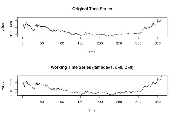
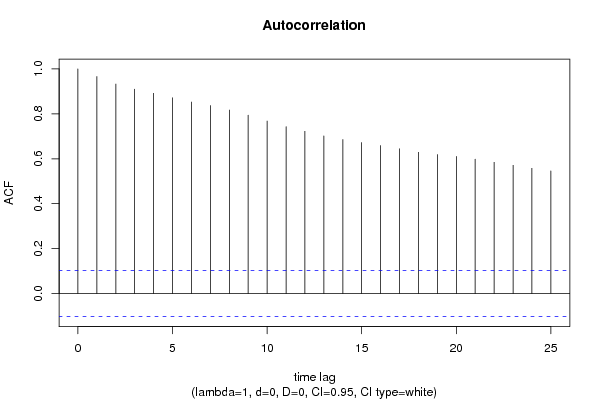
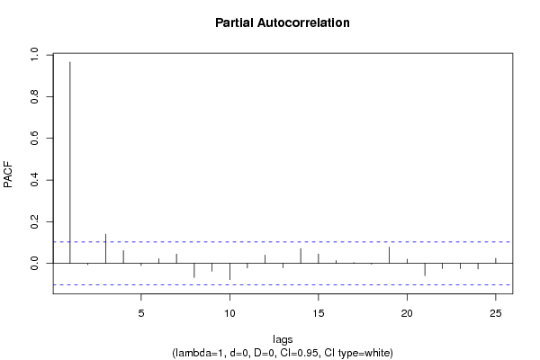
Title produced by software

(Partial) Autocorrelation Function

Date of computation

Fri, 24 Dec 2010 16:13:00 +0000

Cite this page as follows

Statistical Computations at FreeStatistics.org, Office for Research Development and Education, URL https://freestatistics.org/blog/index.php?v=date/2010/Dec/24/t1293207068qv53pnhninyj788.htm/, Retrieved Tue, 30 Apr 2024 03:33:09 +0000

Statistical Computations at FreeStatistics.org, Office for Research Development and Education, URL https://freestatistics.org/blog/index.php?pk=115176, Retrieved Tue, 30 Apr 2024 03:33:09 +0000

QR Codes:

Paste this QR Code to cite your computation.

Original text written by user:

IsPrivate?

No (this computation is public)

User-defined keywords

Estimated Impact

120

Family? (F = Feedback message, R = changed R code, M = changed R Module, P = changed Parameters, D = changed Data)

-     [Univariate Data Series] [data set] [2008-12-01 19:54:57] [b98453cac15ba1066b407e146608df68]
- RMP   [(Partial) Autocorrelation Function] [Unemployment] [2010-11-29 09:05:21] [b98453cac15ba1066b407e146608df68]
- R PD      [(Partial) Autocorrelation Function] [ACF van de goudpr...] [2010-12-24 16:13:00] [03bcd8c83ef1a42b4029a16ba47a4880] [Current]
-    D        [(Partial) Autocorrelation Function] [autocorrelatiefun...] [2010-12-24 16:50:22] [96348ef82925ade81ab3c243141d80f1] 
-    D        [(Partial) Autocorrelation Function] [autocorrelatiefun...] [2010-12-24 16:50:22] [96348ef82925ade81ab3c243141d80f1] 
-    D          [(Partial) Autocorrelation Function] [autocorrelatiefun...] [2010-12-24 16:55:11] [96348ef82925ade81ab3c243141d80f1] 
-   PD            [(Partial) Autocorrelation Function] [ACF goudprijzen m...] [2010-12-28 18:54:34] [30b3e197115d238a51c18bcedc33a6a5] 
-   P           [(Partial) Autocorrelation Function] [ACF inflatie] [2010-12-28 18:50:30] [30b3e197115d238a51c18bcedc33a6a5] 

Feedback Forum

Post a new message

Dataseries X:

Download CSV

Histogram

Boxplots

Summary of computational transaction
Raw Input	view raw input (R code)
Raw Output	view raw output of R engine
Computing time	3 seconds
R Server	'George Udny Yule' @ 72.249.76.132

\begin{tabular}{lllllllll}
\hline
Summary of computational transaction \tabularnewline
Raw Input & view raw input (R code)  \tabularnewline
Raw Output & view raw output of R engine  \tabularnewline
Computing time & 3 seconds \tabularnewline
R Server & 'George Udny Yule' @ 72.249.76.132 \tabularnewline
\hline
\end{tabular}
%Source: https://freestatistics.org/blog/index.php?pk=115176&T=0

[TABLE]
[ROW][C]Summary of computational transaction[/C][/ROW]
[ROW][C]Raw Input[/C][C]view raw input (R code) [/C][/ROW]
[ROW][C]Raw Output[/C][C]view raw output of R engine [/C][/ROW]
[ROW][C]Computing time[/C][C]3 seconds[/C][/ROW]
[ROW][C]R Server[/C][C]'George Udny Yule' @ 72.249.76.132[/C][/ROW]
[/TABLE]
Source: https://freestatistics.org/blog/index.php?pk=115176&T=0

Globally Unique Identifier (entire table): ba.freestatistics.org/blog/index.php?pk=115176&T=0

As an alternative you can also use a QR Code:

The GUIDs for individual cells are displayed in the table below:

Summary of computational transaction
Raw Input	view raw input (R code)
Raw Output	view raw output of R engine
Computing time	3 seconds
R Server	'George Udny Yule' @ 72.249.76.132

Autocorrelation Function
Time lag k	ACF(k)	T-STAT	P-value
1	0.965819	18.3251	0
2	0.932415	17.6913	0
3	0.909618	17.2588	0
4	0.891457	16.9142	0
5	0.871535	16.5362	0
6	0.852397	16.1731	0
7	0.836753	15.8763	0
8	0.816797	15.4976	0
9	0.793975	15.0646	0
10	0.767759	14.5672	0
11	0.742583	14.0895	0
12	0.722255	13.7038	0
13	0.701609	13.3121	0
14	0.685474	13.0059	0
15	0.672259	12.7552	0
16	0.659031	12.5042	0
17	0.644114	12.2212	0
18	0.628411	11.9233	0
19	0.618787	11.7407	0
20	0.610584	11.585	0
21	0.598074	11.3477	0
22	0.584029	11.0812	0
23	0.570787	10.8299	0
24	0.557679	10.5812	0
25	0.545708	10.3541	0

\begin{tabular}{lllllllll}
\hline
Autocorrelation Function \tabularnewline
Time lag k & ACF(k) & T-STAT & P-value \tabularnewline
1 & 0.965819 & 18.3251 & 0 \tabularnewline
2 & 0.932415 & 17.6913 & 0 \tabularnewline
3 & 0.909618 & 17.2588 & 0 \tabularnewline
4 & 0.891457 & 16.9142 & 0 \tabularnewline
5 & 0.871535 & 16.5362 & 0 \tabularnewline
6 & 0.852397 & 16.1731 & 0 \tabularnewline
7 & 0.836753 & 15.8763 & 0 \tabularnewline
8 & 0.816797 & 15.4976 & 0 \tabularnewline
9 & 0.793975 & 15.0646 & 0 \tabularnewline
10 & 0.767759 & 14.5672 & 0 \tabularnewline
11 & 0.742583 & 14.0895 & 0 \tabularnewline
12 & 0.722255 & 13.7038 & 0 \tabularnewline
13 & 0.701609 & 13.3121 & 0 \tabularnewline
14 & 0.685474 & 13.0059 & 0 \tabularnewline
15 & 0.672259 & 12.7552 & 0 \tabularnewline
16 & 0.659031 & 12.5042 & 0 \tabularnewline
17 & 0.644114 & 12.2212 & 0 \tabularnewline
18 & 0.628411 & 11.9233 & 0 \tabularnewline
19 & 0.618787 & 11.7407 & 0 \tabularnewline
20 & 0.610584 & 11.585 & 0 \tabularnewline
21 & 0.598074 & 11.3477 & 0 \tabularnewline
22 & 0.584029 & 11.0812 & 0 \tabularnewline
23 & 0.570787 & 10.8299 & 0 \tabularnewline
24 & 0.557679 & 10.5812 & 0 \tabularnewline
25 & 0.545708 & 10.3541 & 0 \tabularnewline
\hline
\end{tabular}
%Source: https://freestatistics.org/blog/index.php?pk=115176&T=1

[TABLE]
[ROW][C]Autocorrelation Function[/C][/ROW]
[ROW][C]Time lag k[/C][C]ACF(k)[/C][C]T-STAT[/C][C]P-value[/C][/ROW]
[ROW][C]1[/C][C]0.965819[/C][C]18.3251[/C][C]0[/C][/ROW]
[ROW][C]2[/C][C]0.932415[/C][C]17.6913[/C][C]0[/C][/ROW]
[ROW][C]3[/C][C]0.909618[/C][C]17.2588[/C][C]0[/C][/ROW]
[ROW][C]4[/C][C]0.891457[/C][C]16.9142[/C][C]0[/C][/ROW]
[ROW][C]5[/C][C]0.871535[/C][C]16.5362[/C][C]0[/C][/ROW]
[ROW][C]6[/C][C]0.852397[/C][C]16.1731[/C][C]0[/C][/ROW]
[ROW][C]7[/C][C]0.836753[/C][C]15.8763[/C][C]0[/C][/ROW]
[ROW][C]8[/C][C]0.816797[/C][C]15.4976[/C][C]0[/C][/ROW]
[ROW][C]9[/C][C]0.793975[/C][C]15.0646[/C][C]0[/C][/ROW]
[ROW][C]10[/C][C]0.767759[/C][C]14.5672[/C][C]0[/C][/ROW]
[ROW][C]11[/C][C]0.742583[/C][C]14.0895[/C][C]0[/C][/ROW]
[ROW][C]12[/C][C]0.722255[/C][C]13.7038[/C][C]0[/C][/ROW]
[ROW][C]13[/C][C]0.701609[/C][C]13.3121[/C][C]0[/C][/ROW]
[ROW][C]14[/C][C]0.685474[/C][C]13.0059[/C][C]0[/C][/ROW]
[ROW][C]15[/C][C]0.672259[/C][C]12.7552[/C][C]0[/C][/ROW]
[ROW][C]16[/C][C]0.659031[/C][C]12.5042[/C][C]0[/C][/ROW]
[ROW][C]17[/C][C]0.644114[/C][C]12.2212[/C][C]0[/C][/ROW]
[ROW][C]18[/C][C]0.628411[/C][C]11.9233[/C][C]0[/C][/ROW]
[ROW][C]19[/C][C]0.618787[/C][C]11.7407[/C][C]0[/C][/ROW]
[ROW][C]20[/C][C]0.610584[/C][C]11.585[/C][C]0[/C][/ROW]
[ROW][C]21[/C][C]0.598074[/C][C]11.3477[/C][C]0[/C][/ROW]
[ROW][C]22[/C][C]0.584029[/C][C]11.0812[/C][C]0[/C][/ROW]
[ROW][C]23[/C][C]0.570787[/C][C]10.8299[/C][C]0[/C][/ROW]
[ROW][C]24[/C][C]0.557679[/C][C]10.5812[/C][C]0[/C][/ROW]
[ROW][C]25[/C][C]0.545708[/C][C]10.3541[/C][C]0[/C][/ROW]
[/TABLE]
Source: https://freestatistics.org/blog/index.php?pk=115176&T=1

Globally Unique Identifier (entire table): ba.freestatistics.org/blog/index.php?pk=115176&T=1

As an alternative you can also use a QR Code:

The GUIDs for individual cells are displayed in the table below:

Autocorrelation Function
Time lag k	ACF(k)	T-STAT	P-value
1	0.965819	18.3251	0
2	0.932415	17.6913	0
3	0.909618	17.2588	0
4	0.891457	16.9142	0
5	0.871535	16.5362	0
6	0.852397	16.1731	0
7	0.836753	15.8763	0
8	0.816797	15.4976	0
9	0.793975	15.0646	0
10	0.767759	14.5672	0
11	0.742583	14.0895	0
12	0.722255	13.7038	0
13	0.701609	13.3121	0
14	0.685474	13.0059	0
15	0.672259	12.7552	0
16	0.659031	12.5042	0
17	0.644114	12.2212	0
18	0.628411	11.9233	0
19	0.618787	11.7407	0
20	0.610584	11.585	0
21	0.598074	11.3477	0
22	0.584029	11.0812	0
23	0.570787	10.8299	0
24	0.557679	10.5812	0
25	0.545708	10.3541	0

Partial Autocorrelation Function
Time lag k	PACF(k)	T-STAT	P-value
1	0.965819	18.3251	0
2	-0.005829	-0.1106	0.456
3	0.140705	2.6697	0.003968
4	0.061536	1.1676	0.121878
5	-0.010143	-0.1925	0.423747
6	0.022931	0.4351	0.33188
7	0.044937	0.8526	0.197221
8	-0.067344	-1.2778	0.101077
9	-0.037308	-0.7079	0.239744
10	-0.077637	-1.4731	0.070806
11	-0.021941	-0.4163	0.338717
12	0.04018	0.7624	0.223173
13	-0.021113	-0.4006	0.344482
14	0.071218	1.3513	0.08873
15	0.045353	0.8605	0.195038
16	0.014281	0.271	0.393289
17	0.004358	0.0827	0.467077
18	-0.003842	-0.0729	0.470963
19	0.078633	1.492	0.068293
20	0.020804	0.3947	0.34664
21	-0.058432	-1.1087	0.134156
22	-0.024768	-0.4699	0.319343
23	-0.024741	-0.4694	0.319525
24	-0.026342	-0.4998	0.308757
25	0.024847	0.4714	0.318809

\begin{tabular}{lllllllll}
\hline
Partial Autocorrelation Function \tabularnewline
Time lag k & PACF(k) & T-STAT & P-value \tabularnewline
1 & 0.965819 & 18.3251 & 0 \tabularnewline
2 & -0.005829 & -0.1106 & 0.456 \tabularnewline
3 & 0.140705 & 2.6697 & 0.003968 \tabularnewline
4 & 0.061536 & 1.1676 & 0.121878 \tabularnewline
5 & -0.010143 & -0.1925 & 0.423747 \tabularnewline
6 & 0.022931 & 0.4351 & 0.33188 \tabularnewline
7 & 0.044937 & 0.8526 & 0.197221 \tabularnewline
8 & -0.067344 & -1.2778 & 0.101077 \tabularnewline
9 & -0.037308 & -0.7079 & 0.239744 \tabularnewline
10 & -0.077637 & -1.4731 & 0.070806 \tabularnewline
11 & -0.021941 & -0.4163 & 0.338717 \tabularnewline
12 & 0.04018 & 0.7624 & 0.223173 \tabularnewline
13 & -0.021113 & -0.4006 & 0.344482 \tabularnewline
14 & 0.071218 & 1.3513 & 0.08873 \tabularnewline
15 & 0.045353 & 0.8605 & 0.195038 \tabularnewline
16 & 0.014281 & 0.271 & 0.393289 \tabularnewline
17 & 0.004358 & 0.0827 & 0.467077 \tabularnewline
18 & -0.003842 & -0.0729 & 0.470963 \tabularnewline
19 & 0.078633 & 1.492 & 0.068293 \tabularnewline
20 & 0.020804 & 0.3947 & 0.34664 \tabularnewline
21 & -0.058432 & -1.1087 & 0.134156 \tabularnewline
22 & -0.024768 & -0.4699 & 0.319343 \tabularnewline
23 & -0.024741 & -0.4694 & 0.319525 \tabularnewline
24 & -0.026342 & -0.4998 & 0.308757 \tabularnewline
25 & 0.024847 & 0.4714 & 0.318809 \tabularnewline
\hline
\end{tabular}
%Source: https://freestatistics.org/blog/index.php?pk=115176&T=2

[TABLE]
[ROW][C]Partial Autocorrelation Function[/C][/ROW]
[ROW][C]Time lag k[/C][C]PACF(k)[/C][C]T-STAT[/C][C]P-value[/C][/ROW]
[ROW][C]1[/C][C]0.965819[/C][C]18.3251[/C][C]0[/C][/ROW]
[ROW][C]2[/C][C]-0.005829[/C][C]-0.1106[/C][C]0.456[/C][/ROW]
[ROW][C]3[/C][C]0.140705[/C][C]2.6697[/C][C]0.003968[/C][/ROW]
[ROW][C]4[/C][C]0.061536[/C][C]1.1676[/C][C]0.121878[/C][/ROW]
[ROW][C]5[/C][C]-0.010143[/C][C]-0.1925[/C][C]0.423747[/C][/ROW]
[ROW][C]6[/C][C]0.022931[/C][C]0.4351[/C][C]0.33188[/C][/ROW]
[ROW][C]7[/C][C]0.044937[/C][C]0.8526[/C][C]0.197221[/C][/ROW]
[ROW][C]8[/C][C]-0.067344[/C][C]-1.2778[/C][C]0.101077[/C][/ROW]
[ROW][C]9[/C][C]-0.037308[/C][C]-0.7079[/C][C]0.239744[/C][/ROW]
[ROW][C]10[/C][C]-0.077637[/C][C]-1.4731[/C][C]0.070806[/C][/ROW]
[ROW][C]11[/C][C]-0.021941[/C][C]-0.4163[/C][C]0.338717[/C][/ROW]
[ROW][C]12[/C][C]0.04018[/C][C]0.7624[/C][C]0.223173[/C][/ROW]
[ROW][C]13[/C][C]-0.021113[/C][C]-0.4006[/C][C]0.344482[/C][/ROW]
[ROW][C]14[/C][C]0.071218[/C][C]1.3513[/C][C]0.08873[/C][/ROW]
[ROW][C]15[/C][C]0.045353[/C][C]0.8605[/C][C]0.195038[/C][/ROW]
[ROW][C]16[/C][C]0.014281[/C][C]0.271[/C][C]0.393289[/C][/ROW]
[ROW][C]17[/C][C]0.004358[/C][C]0.0827[/C][C]0.467077[/C][/ROW]
[ROW][C]18[/C][C]-0.003842[/C][C]-0.0729[/C][C]0.470963[/C][/ROW]
[ROW][C]19[/C][C]0.078633[/C][C]1.492[/C][C]0.068293[/C][/ROW]
[ROW][C]20[/C][C]0.020804[/C][C]0.3947[/C][C]0.34664[/C][/ROW]
[ROW][C]21[/C][C]-0.058432[/C][C]-1.1087[/C][C]0.134156[/C][/ROW]
[ROW][C]22[/C][C]-0.024768[/C][C]-0.4699[/C][C]0.319343[/C][/ROW]
[ROW][C]23[/C][C]-0.024741[/C][C]-0.4694[/C][C]0.319525[/C][/ROW]
[ROW][C]24[/C][C]-0.026342[/C][C]-0.4998[/C][C]0.308757[/C][/ROW]
[ROW][C]25[/C][C]0.024847[/C][C]0.4714[/C][C]0.318809[/C][/ROW]
[/TABLE]
Source: https://freestatistics.org/blog/index.php?pk=115176&T=2

Globally Unique Identifier (entire table): ba.freestatistics.org/blog/index.php?pk=115176&T=2

As an alternative you can also use a QR Code:

The GUIDs for individual cells are displayed in the table below:

Partial Autocorrelation Function
Time lag k	PACF(k)	T-STAT	P-value
1	0.965819	18.3251	0
2	-0.005829	-0.1106	0.456
3	0.140705	2.6697	0.003968
4	0.061536	1.1676	0.121878
5	-0.010143	-0.1925	0.423747
6	0.022931	0.4351	0.33188
7	0.044937	0.8526	0.197221
8	-0.067344	-1.2778	0.101077
9	-0.037308	-0.7079	0.239744
10	-0.077637	-1.4731	0.070806
11	-0.021941	-0.4163	0.338717
12	0.04018	0.7624	0.223173
13	-0.021113	-0.4006	0.344482
14	0.071218	1.3513	0.08873
15	0.045353	0.8605	0.195038
16	0.014281	0.271	0.393289
17	0.004358	0.0827	0.467077
18	-0.003842	-0.0729	0.470963
19	0.078633	1.492	0.068293
20	0.020804	0.3947	0.34664
21	-0.058432	-1.1087	0.134156
22	-0.024768	-0.4699	0.319343
23	-0.024741	-0.4694	0.319525
24	-0.026342	-0.4998	0.308757
25	0.024847	0.4714	0.318809

Figure 1

PNG link

Postscript link

PDF link

Figure 2

PNG link

Postscript link

PDF link

Figure 3

PNG link

Postscript link

PDF link

Parameters (Session):

par1 = 12 ;

Parameters (R input):

par1 = Default ; par2 = 1 ; par3 = 0 ; par4 = 0 ; par5 = 12 ; par6 = White Noise ; par7 = 0.95 ; par8 = ;

R code (references can be found in the software module):

if (par1 == 'Default') {
par1 = 10*log10(length(x))
} else {
par1 <- as.numeric(par1)
}
par2 <- as.numeric(par2)
par3 <- as.numeric(par3)
par4 <- as.numeric(par4)
par5 <- as.numeric(par5)
if (par6 == 'White Noise') par6 <- 'white' else par6 <- 'ma'
par7 <- as.numeric(par7)
if (par8 != '') par8 <- as.numeric(par8)
ox <- x
if (par8 == '') {
if (par2 == 0) {
x <- log(x)
} else {
x <- (x ^ par2 - 1) / par2
}
} else {
x <- log(x,base=par8)
}
if (par3 > 0) x <- diff(x,lag=1,difference=par3)
if (par4 > 0) x <- diff(x,lag=par5,difference=par4)
bitmap(file='picts.png')
op <- par(mfrow=c(2,1))
plot(ox,type='l',main='Original Time Series',xlab='time',ylab='value')
if (par8=='') {
mytitle <- paste('Working Time Series (lambda=',par2,', d=',par3,', D=',par4,')',sep='')
mysub <- paste('(lambda=',par2,', d=',par3,', D=',par4,', CI=', par7, ', CI type=',par6,')',sep='')
} else {
mytitle <- paste('Working Time Series (base=',par8,', d=',par3,', D=',par4,')',sep='')
mysub <- paste('(base=',par8,', d=',par3,', D=',par4,', CI=', par7, ', CI type=',par6,')',sep='')
}
plot(x,type='l', main=mytitle,xlab='time',ylab='value')
par(op)
dev.off()
bitmap(file='pic1.png')
racf <- acf(x, par1, main='Autocorrelation', xlab='time lag', ylab='ACF', ci.type=par6, ci=par7, sub=mysub)
dev.off()
bitmap(file='pic2.png')
rpacf <- pacf(x,par1,main='Partial Autocorrelation',xlab='lags',ylab='PACF',sub=mysub)
dev.off()
(myacf <- c(racf$acf))
(mypacf <- c(rpacf$acf))
lengthx <- length(x)
sqrtn <- sqrt(lengthx)
load(file='createtable')
a<-table.start()
a<-table.row.start(a)
a<-table.element(a,'Autocorrelation Function',4,TRUE)
a<-table.row.end(a)
a<-table.row.start(a)
a<-table.element(a,'Time lag k',header=TRUE)
a<-table.element(a,hyperlink('basics.htm','ACF(k)','click here for more information about the Autocorrelation Function'),header=TRUE)
a<-table.element(a,'T-STAT',header=TRUE)
a<-table.element(a,'P-value',header=TRUE)
a<-table.row.end(a)
for (i in 2:(par1+1)) {
a<-table.row.start(a)
a<-table.element(a,i-1,header=TRUE)
a<-table.element(a,round(myacf[i],6))
mytstat <- myacf[i]*sqrtn
a<-table.element(a,round(mytstat,4))
a<-table.element(a,round(1-pt(abs(mytstat),lengthx),6))
a<-table.row.end(a)
}
a<-table.end(a)
table.save(a,file='mytable.tab')
a<-table.start()
a<-table.row.start(a)
a<-table.element(a,'Partial Autocorrelation Function',4,TRUE)
a<-table.row.end(a)
a<-table.row.start(a)
a<-table.element(a,'Time lag k',header=TRUE)
a<-table.element(a,hyperlink('basics.htm','PACF(k)','click here for more information about the Partial Autocorrelation Function'),header=TRUE)
a<-table.element(a,'T-STAT',header=TRUE)
a<-table.element(a,'P-value',header=TRUE)
a<-table.row.end(a)
for (i in 1:par1) {
a<-table.row.start(a)
a<-table.element(a,i,header=TRUE)
a<-table.element(a,round(mypacf[i],6))
mytstat <- mypacf[i]*sqrtn
a<-table.element(a,round(mytstat,4))
a<-table.element(a,round(1-pt(abs(mytstat),lengthx),6))
a<-table.row.end(a)
}
a<-table.end(a)
table.save(a,file='mytable1.tab')

Free Statistics

Description of Statistical Computation

Tree of Dependent Computations

Dataset

Tables (Output of Computation)

Figures (Output of Computation)

Input Parameters & R Code