Free Statistics
of Irreproducible Research!
Description of Statistical Computation | |||||||||||||||||||||||||||||||||||||||||||||||||||||
|---|---|---|---|---|---|---|---|---|---|---|---|---|---|---|---|---|---|---|---|---|---|---|---|---|---|---|---|---|---|---|---|---|---|---|---|---|---|---|---|---|---|---|---|---|---|---|---|---|---|---|---|---|---|
| Author's title | |||||||||||||||||||||||||||||||||||||||||||||||||||||
| Author | *The author of this computation has been verified* | ||||||||||||||||||||||||||||||||||||||||||||||||||||
| R Software Module | rwasp_edauni.wasp | ||||||||||||||||||||||||||||||||||||||||||||||||||||
| Title produced by software | Univariate Explorative Data Analysis | ||||||||||||||||||||||||||||||||||||||||||||||||||||
| Date of computation | Fri, 24 Dec 2010 15:16:17 +0000 | ||||||||||||||||||||||||||||||||||||||||||||||||||||
| Cite this page as follows | Statistical Computations at FreeStatistics.org, Office for Research Development and Education, URL https://freestatistics.org/blog/index.php?v=date/2010/Dec/24/t12932036449y2cpyxx6gol1g4.htm/, Retrieved Tue, 30 Apr 2024 06:19:03 +0000 | ||||||||||||||||||||||||||||||||||||||||||||||||||||
| Statistical Computations at FreeStatistics.org, Office for Research Development and Education, URL https://freestatistics.org/blog/index.php?pk=115093, Retrieved Tue, 30 Apr 2024 06:19:03 +0000 | |||||||||||||||||||||||||||||||||||||||||||||||||||||
| QR Codes: | |||||||||||||||||||||||||||||||||||||||||||||||||||||
|
| |||||||||||||||||||||||||||||||||||||||||||||||||||||
| Original text written by user: | |||||||||||||||||||||||||||||||||||||||||||||||||||||
| IsPrivate? | No (this computation is public) | ||||||||||||||||||||||||||||||||||||||||||||||||||||
| User-defined keywords | |||||||||||||||||||||||||||||||||||||||||||||||||||||
| Estimated Impact | 171 | ||||||||||||||||||||||||||||||||||||||||||||||||||||
Tree of Dependent Computations | |||||||||||||||||||||||||||||||||||||||||||||||||||||
| Family? (F = Feedback message, R = changed R code, M = changed R Module, P = changed Parameters, D = changed Data) | |||||||||||||||||||||||||||||||||||||||||||||||||||||
| - [Multiple Regression] [Competence to learn] [2010-11-17 07:43:53] [b98453cac15ba1066b407e146608df68] - PD [Multiple Regression] [Mini-Tutorial FMPS] [2010-11-22 11:26:18] [3cdf9c5e1f396891d2638627ccb7b98d] - D [Multiple Regression] [Mini-Tutorial FMPS] [2010-11-22 22:19:35] [3cdf9c5e1f396891d2638627ccb7b98d] - D [Multiple Regression] [Mini-Tutorial FMP...] [2010-11-22 23:58:11] [3cdf9c5e1f396891d2638627ccb7b98d] - D [Multiple Regression] [] [2010-11-24 15:02:47] [afdb2fc47981b6a655b732edc8065db9] - RMPD [Univariate Explorative Data Analysis] [Univariate EDA (Pop)] [2010-12-17 16:23:24] [1251ac2db27b84d4a3ba43449388906b] - [Univariate Explorative Data Analysis] [] [2010-12-24 15:16:17] [4f70e6cd0867f10d298e58e8e27859b5] [Current] | |||||||||||||||||||||||||||||||||||||||||||||||||||||
| Feedback Forum | |||||||||||||||||||||||||||||||||||||||||||||||||||||
Post a new message | |||||||||||||||||||||||||||||||||||||||||||||||||||||
Dataset | |||||||||||||||||||||||||||||||||||||||||||||||||||||
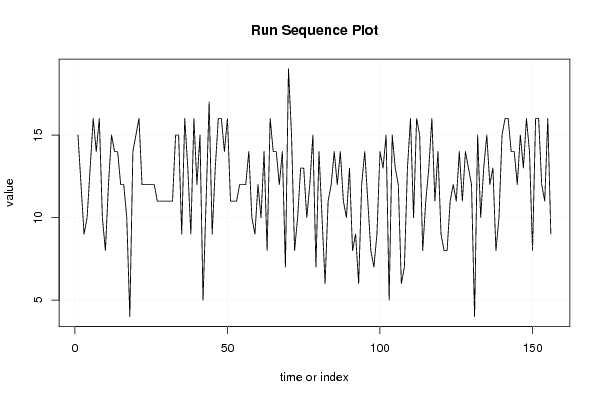
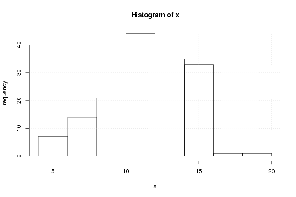
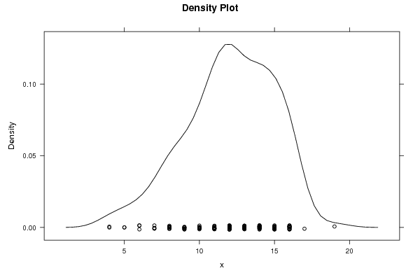
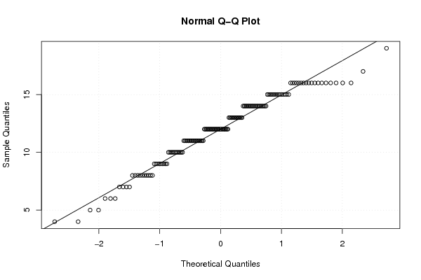
| Dataseries X: | |||||||||||||||||||||||||||||||||||||||||||||||||||||
15 12 9 10 13 16 14 16 10 8 12 15 14 14 12 12 10 4 14 15 16 12 12 12 12 12 11 11 11 11 11 11 15 15 9 16 13 9 16 12 15 5 11 17 9 13 16 16 14 16 11 11 11 12 12 12 14 10 9 12 10 14 8 16 14 14 12 14 7 19 15 8 10 13 13 10 12 15 7 14 10 6 11 12 14 12 14 11 10 13 8 9 6 12 14 11 8 7 9 14 13 15 5 15 13 12 6 7 13 16 10 16 15 8 11 13 16 11 14 9 8 8 11 12 11 14 11 14 13 12 4 15 10 13 15 12 13 8 10 15 16 16 14 14 12 15 13 16 14 8 16 16 12 11 16 9 | |||||||||||||||||||||||||||||||||||||||||||||||||||||
Tables (Output of Computation) | |||||||||||||||||||||||||||||||||||||||||||||||||||||
| |||||||||||||||||||||||||||||||||||||||||||||||||||||
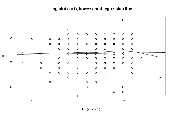
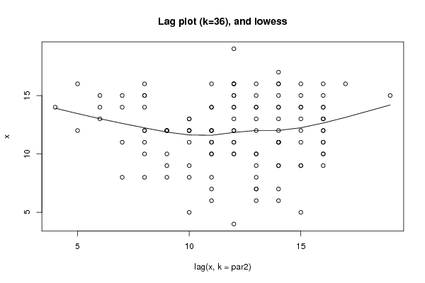
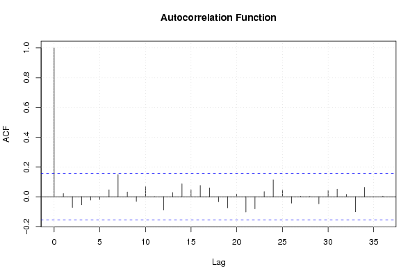
Figures (Output of Computation) | |||||||||||||||||||||||||||||||||||||||||||||||||||||
Input Parameters & R Code | |||||||||||||||||||||||||||||||||||||||||||||||||||||
| Parameters (Session): | |||||||||||||||||||||||||||||||||||||||||||||||||||||
| par1 = 0 ; par2 = 36 ; | |||||||||||||||||||||||||||||||||||||||||||||||||||||
| Parameters (R input): | |||||||||||||||||||||||||||||||||||||||||||||||||||||
| par1 = 0 ; par2 = 36 ; | |||||||||||||||||||||||||||||||||||||||||||||||||||||
| R code (references can be found in the software module): | |||||||||||||||||||||||||||||||||||||||||||||||||||||
par1 <- as.numeric(par1) | |||||||||||||||||||||||||||||||||||||||||||||||||||||