\begin{tabular}{lllllllll}
\hline
Summary of computational transaction \tabularnewline
Raw Input & view raw input (R code)  \tabularnewline
Raw Output & view raw output of R engine  \tabularnewline
Computing time & 6 seconds \tabularnewline
R Server & 'Sir Ronald Aylmer Fisher' @ 193.190.124.24 \tabularnewline
\hline
\end{tabular}
%Source: https://freestatistics.org/blog/index.php?pk=114949&T=0
[TABLE]
[ROW][C]Summary of computational transaction[/C][/ROW]
[ROW][C]Raw Input[/C][C]view raw input (R code) [/C][/ROW]
[ROW][C]Raw Output[/C][C]view raw output of R engine [/C][/ROW]
[ROW][C]Computing time[/C][C]6 seconds[/C][/ROW]
[ROW][C]R Server[/C][C]'Sir Ronald Aylmer Fisher' @ 193.190.124.24[/C][/ROW]
[/TABLE]
Source: https://freestatistics.org/blog/index.php?pk=114949&T=0
If you paste this QR Code into your document, anyone with a smartphone or tablet will be able to scan it and view this table in a browser.
If you paste this QR Code into your document, anyone with a smartphone or tablet will be able to scan it and view this table in a browser.
If you paste this QR Code into your document, anyone with a smartphone or tablet will be able to scan it and view this table in a browser.
If you paste this QR Code into your document, anyone with a smartphone or tablet will be able to scan it and view this table in a browser.
If you paste this QR Code into your document, anyone with a smartphone or tablet will be able to scan it and view this table in a browser.
| Multiple Linear Regression - Estimated Regression Equation | | Unemployment[t] = + 64.1172982454136 -0.281097416377750CPI[t] + 0.324336594244599Inflation[t] -0.000372199226350419Import[t] -0.000187128262761976Export[t] + 0.0426951769815421M1[t] -0.916417283203493M2[t] -0.437903256624127M3[t] + 0.219798810633657M4[t] + 0.830300978554858M5[t] + 1.50462169015839M6[t] + 1.87395398377241M7[t] + 2.13375114434699M8[t] + 2.30170282119335M9[t] + 2.69717334939725M10[t] + 1.28684872932107M11[t] + 0.270121808499834t + e[t] |
\begin{tabular}{lllllllll}
\hline
Multiple Linear Regression - Estimated Regression Equation \tabularnewline
Unemployment[t] =  +  64.1172982454136 -0.281097416377750CPI[t] +  0.324336594244599Inflation[t] -0.000372199226350419Import[t] -0.000187128262761976Export[t] +  0.0426951769815421M1[t] -0.916417283203493M2[t] -0.437903256624127M3[t] +  0.219798810633657M4[t] +  0.830300978554858M5[t] +  1.50462169015839M6[t] +  1.87395398377241M7[t] +  2.13375114434699M8[t] +  2.30170282119335M9[t] +  2.69717334939725M10[t] +  1.28684872932107M11[t] +  0.270121808499834t  + e[t] \tabularnewline
\hline
\end{tabular}
%Source: https://freestatistics.org/blog/index.php?pk=114949&T=1
[TABLE]
[ROW][C]Multiple Linear Regression - Estimated Regression Equation[/C][/ROW]
[ROW][C]Unemployment[t] =  +  64.1172982454136 -0.281097416377750CPI[t] +  0.324336594244599Inflation[t] -0.000372199226350419Import[t] -0.000187128262761976Export[t] +  0.0426951769815421M1[t] -0.916417283203493M2[t] -0.437903256624127M3[t] +  0.219798810633657M4[t] +  0.830300978554858M5[t] +  1.50462169015839M6[t] +  1.87395398377241M7[t] +  2.13375114434699M8[t] +  2.30170282119335M9[t] +  2.69717334939725M10[t] +  1.28684872932107M11[t] +  0.270121808499834t  + e[t][/C][/ROW]
[/TABLE]
Source: https://freestatistics.org/blog/index.php?pk=114949&T=1
Globally Unique Identifier (entire table): ba.freestatistics.org/blog/index.php?pk=114949&T=1
As an alternative you can also use a QR Code:
The GUIDs for individual cells are displayed in the table below:
| Multiple Linear Regression - Estimated Regression Equation | | Unemployment[t] = + 64.1172982454136 -0.281097416377750CPI[t] + 0.324336594244599Inflation[t] -0.000372199226350419Import[t] -0.000187128262761976Export[t] + 0.0426951769815421M1[t] -0.916417283203493M2[t] -0.437903256624127M3[t] + 0.219798810633657M4[t] + 0.830300978554858M5[t] + 1.50462169015839M6[t] + 1.87395398377241M7[t] + 2.13375114434699M8[t] + 2.30170282119335M9[t] + 2.69717334939725M10[t] + 1.28684872932107M11[t] + 0.270121808499834t + e[t] |
If you paste this QR Code into your document, anyone with a smartphone or tablet will be able to scan it and view this table in a browser.
If you paste this QR Code into your document, anyone with a smartphone or tablet will be able to scan it and view this table in a browser.
If you paste this QR Code into your document, anyone with a smartphone or tablet will be able to scan it and view this table in a browser.
If you paste this QR Code into your document, anyone with a smartphone or tablet will be able to scan it and view this table in a browser.
If you paste this QR Code into your document, anyone with a smartphone or tablet will be able to scan it and view this table in a browser.
| Multiple Linear Regression - Ordinary Least Squares | | Variable | Parameter | S.D. | T-STATH0: parameter = 0 | 2-tail p-value | 1-tail p-value | | (Intercept) | 64.1172982454136 | 7.36321 | 8.7078 | 0 | 0 | | CPI | -0.281097416377750 | 0.038559 | -7.29 | 0 | 0 | | Inflation | 0.324336594244599 | 0.086058 | 3.7688 | 0.000414 | 0.000207 | | Import | -0.000372199226350419 | 4.1e-05 | -8.9983 | 0 | 0 | | Export | -0.000187128262761976 | 0.000172 | -1.0851 | 0.282768 | 0.141384 | | M1 | 0.0426951769815421 | 0.390394 | 0.1094 | 0.913327 | 0.456663 | | M2 | -0.916417283203493 | 0.384878 | -2.3811 | 0.020888 | 0.010444 | | M3 | -0.437903256624127 | 0.370184 | -1.1829 | 0.242115 | 0.121057 | | M4 | 0.219798810633657 | 0.374921 | 0.5863 | 0.560193 | 0.280097 | | M5 | 0.830300978554858 | 0.369454 | 2.2474 | 0.028803 | 0.014401 | | M6 | 1.50462169015839 | 0.381186 | 3.9472 | 0.000234 | 0.000117 | | M7 | 1.87395398377241 | 0.395099 | 4.743 | 1.6e-05 | 8e-06 | | M8 | 2.13375114434699 | 0.402045 | 5.3072 | 2e-06 | 1e-06 | | M9 | 2.30170282119335 | 0.433819 | 5.3057 | 2e-06 | 1e-06 | | M10 | 2.69717334939725 | 0.426883 | 6.3183 | 0 | 0 | | M11 | 1.28684872932107 | 0.396709 | 3.2438 | 0.002044 | 0.001022 | | t | 0.270121808499834 | 0.023213 | 11.6364 | 0 | 0 |
\begin{tabular}{lllllllll}
\hline
Multiple Linear Regression - Ordinary Least Squares \tabularnewline
Variable & Parameter & S.D. & T-STATH0: parameter = 0 & 2-tail p-value & 1-tail p-value \tabularnewline
(Intercept) & 64.1172982454136 & 7.36321 & 8.7078 & 0 & 0 \tabularnewline
CPI & -0.281097416377750 & 0.038559 & -7.29 & 0 & 0 \tabularnewline
Inflation & 0.324336594244599 & 0.086058 & 3.7688 & 0.000414 & 0.000207 \tabularnewline
Import & -0.000372199226350419 & 4.1e-05 & -8.9983 & 0 & 0 \tabularnewline
Export & -0.000187128262761976 & 0.000172 & -1.0851 & 0.282768 & 0.141384 \tabularnewline
M1 & 0.0426951769815421 & 0.390394 & 0.1094 & 0.913327 & 0.456663 \tabularnewline
M2 & -0.916417283203493 & 0.384878 & -2.3811 & 0.020888 & 0.010444 \tabularnewline
M3 & -0.437903256624127 & 0.370184 & -1.1829 & 0.242115 & 0.121057 \tabularnewline
M4 & 0.219798810633657 & 0.374921 & 0.5863 & 0.560193 & 0.280097 \tabularnewline
M5 & 0.830300978554858 & 0.369454 & 2.2474 & 0.028803 & 0.014401 \tabularnewline
M6 & 1.50462169015839 & 0.381186 & 3.9472 & 0.000234 & 0.000117 \tabularnewline
M7 & 1.87395398377241 & 0.395099 & 4.743 & 1.6e-05 & 8e-06 \tabularnewline
M8 & 2.13375114434699 & 0.402045 & 5.3072 & 2e-06 & 1e-06 \tabularnewline
M9 & 2.30170282119335 & 0.433819 & 5.3057 & 2e-06 & 1e-06 \tabularnewline
M10 & 2.69717334939725 & 0.426883 & 6.3183 & 0 & 0 \tabularnewline
M11 & 1.28684872932107 & 0.396709 & 3.2438 & 0.002044 & 0.001022 \tabularnewline
t & 0.270121808499834 & 0.023213 & 11.6364 & 0 & 0 \tabularnewline
\hline
\end{tabular}
%Source: https://freestatistics.org/blog/index.php?pk=114949&T=2
[TABLE]
[ROW][C]Multiple Linear Regression - Ordinary Least Squares[/C][/ROW]
[ROW][C]Variable[/C][C]Parameter[/C][C]S.D.[/C][C]T-STATH0: parameter = 0[/C][C]2-tail p-value[/C][C]1-tail p-value[/C][/ROW]
[ROW][C](Intercept)[/C][C]64.1172982454136[/C][C]7.36321[/C][C]8.7078[/C][C]0[/C][C]0[/C][/ROW]
[ROW][C]CPI[/C][C]-0.281097416377750[/C][C]0.038559[/C][C]-7.29[/C][C]0[/C][C]0[/C][/ROW]
[ROW][C]Inflation[/C][C]0.324336594244599[/C][C]0.086058[/C][C]3.7688[/C][C]0.000414[/C][C]0.000207[/C][/ROW]
[ROW][C]Import[/C][C]-0.000372199226350419[/C][C]4.1e-05[/C][C]-8.9983[/C][C]0[/C][C]0[/C][/ROW]
[ROW][C]Export[/C][C]-0.000187128262761976[/C][C]0.000172[/C][C]-1.0851[/C][C]0.282768[/C][C]0.141384[/C][/ROW]
[ROW][C]M1[/C][C]0.0426951769815421[/C][C]0.390394[/C][C]0.1094[/C][C]0.913327[/C][C]0.456663[/C][/ROW]
[ROW][C]M2[/C][C]-0.916417283203493[/C][C]0.384878[/C][C]-2.3811[/C][C]0.020888[/C][C]0.010444[/C][/ROW]
[ROW][C]M3[/C][C]-0.437903256624127[/C][C]0.370184[/C][C]-1.1829[/C][C]0.242115[/C][C]0.121057[/C][/ROW]
[ROW][C]M4[/C][C]0.219798810633657[/C][C]0.374921[/C][C]0.5863[/C][C]0.560193[/C][C]0.280097[/C][/ROW]
[ROW][C]M5[/C][C]0.830300978554858[/C][C]0.369454[/C][C]2.2474[/C][C]0.028803[/C][C]0.014401[/C][/ROW]
[ROW][C]M6[/C][C]1.50462169015839[/C][C]0.381186[/C][C]3.9472[/C][C]0.000234[/C][C]0.000117[/C][/ROW]
[ROW][C]M7[/C][C]1.87395398377241[/C][C]0.395099[/C][C]4.743[/C][C]1.6e-05[/C][C]8e-06[/C][/ROW]
[ROW][C]M8[/C][C]2.13375114434699[/C][C]0.402045[/C][C]5.3072[/C][C]2e-06[/C][C]1e-06[/C][/ROW]
[ROW][C]M9[/C][C]2.30170282119335[/C][C]0.433819[/C][C]5.3057[/C][C]2e-06[/C][C]1e-06[/C][/ROW]
[ROW][C]M10[/C][C]2.69717334939725[/C][C]0.426883[/C][C]6.3183[/C][C]0[/C][C]0[/C][/ROW]
[ROW][C]M11[/C][C]1.28684872932107[/C][C]0.396709[/C][C]3.2438[/C][C]0.002044[/C][C]0.001022[/C][/ROW]
[ROW][C]t[/C][C]0.270121808499834[/C][C]0.023213[/C][C]11.6364[/C][C]0[/C][C]0[/C][/ROW]
[/TABLE]
Source: https://freestatistics.org/blog/index.php?pk=114949&T=2
Globally Unique Identifier (entire table): ba.freestatistics.org/blog/index.php?pk=114949&T=2
As an alternative you can also use a QR Code:
The GUIDs for individual cells are displayed in the table below:
| Multiple Linear Regression - Ordinary Least Squares | | Variable | Parameter | S.D. | T-STATH0: parameter = 0 | 2-tail p-value | 1-tail p-value | | (Intercept) | 64.1172982454136 | 7.36321 | 8.7078 | 0 | 0 | | CPI | -0.281097416377750 | 0.038559 | -7.29 | 0 | 0 | | Inflation | 0.324336594244599 | 0.086058 | 3.7688 | 0.000414 | 0.000207 | | Import | -0.000372199226350419 | 4.1e-05 | -8.9983 | 0 | 0 | | Export | -0.000187128262761976 | 0.000172 | -1.0851 | 0.282768 | 0.141384 | | M1 | 0.0426951769815421 | 0.390394 | 0.1094 | 0.913327 | 0.456663 | | M2 | -0.916417283203493 | 0.384878 | -2.3811 | 0.020888 | 0.010444 | | M3 | -0.437903256624127 | 0.370184 | -1.1829 | 0.242115 | 0.121057 | | M4 | 0.219798810633657 | 0.374921 | 0.5863 | 0.560193 | 0.280097 | | M5 | 0.830300978554858 | 0.369454 | 2.2474 | 0.028803 | 0.014401 | | M6 | 1.50462169015839 | 0.381186 | 3.9472 | 0.000234 | 0.000117 | | M7 | 1.87395398377241 | 0.395099 | 4.743 | 1.6e-05 | 8e-06 | | M8 | 2.13375114434699 | 0.402045 | 5.3072 | 2e-06 | 1e-06 | | M9 | 2.30170282119335 | 0.433819 | 5.3057 | 2e-06 | 1e-06 | | M10 | 2.69717334939725 | 0.426883 | 6.3183 | 0 | 0 | | M11 | 1.28684872932107 | 0.396709 | 3.2438 | 0.002044 | 0.001022 | | t | 0.270121808499834 | 0.023213 | 11.6364 | 0 | 0 |
If you paste this QR Code into your document, anyone with a smartphone or tablet will be able to scan it and view this table in a browser.
If you paste this QR Code into your document, anyone with a smartphone or tablet will be able to scan it and view this table in a browser.
If you paste this QR Code into your document, anyone with a smartphone or tablet will be able to scan it and view this table in a browser.
If you paste this QR Code into your document, anyone with a smartphone or tablet will be able to scan it and view this table in a browser.
If you paste this QR Code into your document, anyone with a smartphone or tablet will be able to scan it and view this table in a browser.
| Multiple Linear Regression - Regression Statistics | | Multiple R | 0.972181032463087 | | R-squared | 0.945135959880994 | | Adjusted R-squared | 0.928573230788463 | | F-TEST (value) | 57.0640233623845 | | F-TEST (DF numerator) | 16 | | F-TEST (DF denominator) | 53 | | p-value | 0 | | Multiple Linear Regression - Residual Statistics | | Residual Standard Deviation | 0.577145210441974 | | Sum Squared Residuals | 17.6541194786139 |
\begin{tabular}{lllllllll}
\hline
Multiple Linear Regression - Regression Statistics \tabularnewline
Multiple R & 0.972181032463087 \tabularnewline
R-squared & 0.945135959880994 \tabularnewline
Adjusted R-squared & 0.928573230788463 \tabularnewline
F-TEST (value) & 57.0640233623845 \tabularnewline
F-TEST (DF numerator) & 16 \tabularnewline
F-TEST (DF denominator) & 53 \tabularnewline
p-value & 0 \tabularnewline
Multiple Linear Regression - Residual Statistics \tabularnewline
Residual Standard Deviation & 0.577145210441974 \tabularnewline
Sum Squared Residuals & 17.6541194786139 \tabularnewline
\hline
\end{tabular}
%Source: https://freestatistics.org/blog/index.php?pk=114949&T=3
[TABLE]
[ROW][C]Multiple Linear Regression - Regression Statistics[/C][/ROW]
[ROW][C]Multiple R[/C][C]0.972181032463087[/C][/ROW]
[ROW][C]R-squared[/C][C]0.945135959880994[/C][/ROW]
[ROW][C]Adjusted R-squared[/C][C]0.928573230788463[/C][/ROW]
[ROW][C]F-TEST (value)[/C][C]57.0640233623845[/C][/ROW]
[ROW][C]F-TEST (DF numerator)[/C][C]16[/C][/ROW]
[ROW][C]F-TEST (DF denominator)[/C][C]53[/C][/ROW]
[ROW][C]p-value[/C][C]0[/C][/ROW]
[ROW][C]Multiple Linear Regression - Residual Statistics[/C][/ROW]
[ROW][C]Residual Standard Deviation[/C][C]0.577145210441974[/C][/ROW]
[ROW][C]Sum Squared Residuals[/C][C]17.6541194786139[/C][/ROW]
[/TABLE]
Source: https://freestatistics.org/blog/index.php?pk=114949&T=3
Globally Unique Identifier (entire table): ba.freestatistics.org/blog/index.php?pk=114949&T=3
As an alternative you can also use a QR Code:
The GUIDs for individual cells are displayed in the table below:
| Multiple Linear Regression - Regression Statistics | | Multiple R | 0.972181032463087 | | R-squared | 0.945135959880994 | | Adjusted R-squared | 0.928573230788463 | | F-TEST (value) | 57.0640233623845 | | F-TEST (DF numerator) | 16 | | F-TEST (DF denominator) | 53 | | p-value | 0 | | Multiple Linear Regression - Residual Statistics | | Residual Standard Deviation | 0.577145210441974 | | Sum Squared Residuals | 17.6541194786139 |
If you paste this QR Code into your document, anyone with a smartphone or tablet will be able to scan it and view this table in a browser.
If you paste this QR Code into your document, anyone with a smartphone or tablet will be able to scan it and view this table in a browser.
If you paste this QR Code into your document, anyone with a smartphone or tablet will be able to scan it and view this table in a browser.
If you paste this QR Code into your document, anyone with a smartphone or tablet will be able to scan it and view this table in a browser.
If you paste this QR Code into your document, anyone with a smartphone or tablet will be able to scan it and view this table in a browser.
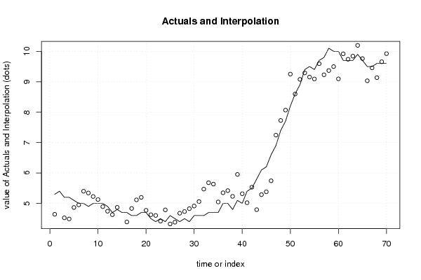
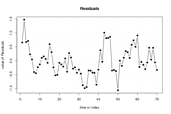
| Multiple Linear Regression - Actuals, Interpolation, and Residuals | | Time or Index | Actuals | InterpolationForecast | ResidualsPrediction Error | | 1 | 5.3 | 4.64276291388123 | 0.657237086118774 | | 2 | 5.4 | 3.92647471004821 | 1.47352528995179 | | 3 | 5.2 | 4.52694810590232 | 0.673051894097676 | | 4 | 5.2 | 4.48886033813804 | 0.71113966186196 | | 5 | 5.1 | 4.86633100896242 | 0.233668991037578 | | 6 | 5 | 4.95151013786072 | 0.0484898621392773 | | 7 | 5 | 5.39995763441057 | -0.399957634410571 | | 8 | 4.9 | 5.34214081708817 | -0.442140817088167 | | 9 | 5 | 5.22646406174412 | -0.22646406174412 | | 10 | 5 | 5.12700148398417 | -0.127001483984166 | | 11 | 5 | 4.8933740775523 | 0.106625922447701 | | 12 | 4.9 | 4.74285877550726 | 0.157141224492744 | | 13 | 4.7 | 4.62985632300701 | 0.0701436769929925 | | 14 | 4.8 | 4.8697416471152 | -0.069741647115198 | | 15 | 4.7 | 4.10522333701710 | 0.594776662982895 | | 16 | 4.7 | 4.39024942400613 | 0.309750575993868 | | 17 | 4.6 | 4.83358786606014 | -0.233587866060143 | | 18 | 4.6 | 5.11643881044293 | -0.516438810442934 | | 19 | 4.7 | 5.1988333111493 | -0.498833311149298 | | 20 | 4.7 | 4.77261102510945 | -0.072611025109454 | | 21 | 4.5 | 4.62849147600372 | -0.128491476003723 | | 22 | 4.4 | 4.60398180964456 | -0.203981809644562 | | 23 | 4.5 | 4.41688745896897 | 0.0831125410310287 | | 24 | 4.4 | 4.78662888531707 | -0.386628885317066 | | 25 | 4.6 | 4.32423312484676 | 0.275766875153238 | | 26 | 4.5 | 4.38260494758344 | 0.117395052416563 | | 27 | 4.4 | 4.67769420513175 | -0.277694205131751 | | 28 | 4.5 | 4.73223324619346 | -0.232233246193464 | | 29 | 4.4 | 4.82667300569558 | -0.426673005695582 | | 30 | 4.6 | 4.91425550358615 | -0.314255503586154 | | 31 | 4.6 | 5.05968564711435 | -0.459685647114347 | | 32 | 4.6 | 5.4702961045422 | -0.870296104542199 | | 33 | 4.7 | 5.67845374765104 | -0.978453747651043 | | 34 | 4.7 | 5.63513740691565 | -0.935137406915654 | | 35 | 4.7 | 5.04727941261672 | -0.347279412616722 | | 36 | 5 | 5.34954875882431 | -0.349548758824314 | | 37 | 5 | 5.4197883577543 | -0.419788357754304 | | 38 | 4.8 | 5.23147990249331 | -0.43147990249331 | | 39 | 5.1 | 5.95275082479054 | -0.852750824790536 | | 40 | 5 | 5.31696339784819 | -0.316963397848187 | | 41 | 5.4 | 5.02372447246324 | 0.376275527536764 | | 42 | 5.5 | 5.53313960384875 | -0.0331396038487539 | | 43 | 5.8 | 4.79457207377784 | 1.00542792622216 | | 44 | 6.1 | 5.28839289483726 | 0.811607105162739 | | 45 | 6.2 | 5.38165707431945 | 0.818342925680552 | | 46 | 6.6 | 5.74382693902568 | 0.85617306097432 | | 47 | 6.9 | 7.24507079386054 | -0.345070793860542 | | 48 | 7.4 | 7.72686078687294 | -0.326860786872942 | | 49 | 7.7 | 8.06605007148066 | -0.366050071480658 | | 50 | 8.2 | 9.25129175367216 | -1.05129175367216 | | 51 | 8.6 | 8.59654734022549 | 0.00345265977451100 | | 52 | 8.9 | 9.07753477334944 | -0.177534773349438 | | 53 | 9.4 | 9.28937457609635 | 0.110625423903649 | | 54 | 9.5 | 9.15299374181268 | 0.347006258187322 | | 55 | 9.4 | 9.09143661986234 | 0.308563380137658 | | 56 | 9.7 | 9.59286612456255 | 0.107133875437446 | | 57 | 9.8 | 9.22847058190075 | 0.571529418099255 | | 58 | 10.1 | 9.36765796990535 | 0.732342030094653 | | 59 | 10 | 9.49738825700147 | 0.502611742998533 | | 60 | 10 | 9.09410279347842 | 0.905897206521578 | | 61 | 9.7 | 9.91730920903004 | -0.217309209030043 | | 62 | 9.7 | 9.73840703908768 | -0.0384070390876845 | | 63 | 9.7 | 9.8408361869328 | -0.140836186932795 | | 64 | 9.9 | 10.1941588204647 | -0.294158820464739 | | 65 | 9.7 | 9.76030907072226 | -0.0603090707222659 | | 66 | 9.5 | 9.03166220244876 | 0.468337797551243 | | 67 | 9.5 | 9.4555147136856 | 0.0444852863144009 | | 68 | 9.6 | 9.13369303386036 | 0.466306966139635 | | 69 | 9.6 | 9.65646305838092 | -0.056463058380921 | | 70 | 9.6 | 9.9223943905246 | -0.322394390524591 |
\begin{tabular}{lllllllll}
\hline
Multiple Linear Regression - Actuals, Interpolation, and Residuals \tabularnewline
Time or Index & Actuals & InterpolationForecast & ResidualsPrediction Error \tabularnewline
1 & 5.3 & 4.64276291388123 & 0.657237086118774 \tabularnewline
2 & 5.4 & 3.92647471004821 & 1.47352528995179 \tabularnewline
3 & 5.2 & 4.52694810590232 & 0.673051894097676 \tabularnewline
4 & 5.2 & 4.48886033813804 & 0.71113966186196 \tabularnewline
5 & 5.1 & 4.86633100896242 & 0.233668991037578 \tabularnewline
6 & 5 & 4.95151013786072 & 0.0484898621392773 \tabularnewline
7 & 5 & 5.39995763441057 & -0.399957634410571 \tabularnewline
8 & 4.9 & 5.34214081708817 & -0.442140817088167 \tabularnewline
9 & 5 & 5.22646406174412 & -0.22646406174412 \tabularnewline
10 & 5 & 5.12700148398417 & -0.127001483984166 \tabularnewline
11 & 5 & 4.8933740775523 & 0.106625922447701 \tabularnewline
12 & 4.9 & 4.74285877550726 & 0.157141224492744 \tabularnewline
13 & 4.7 & 4.62985632300701 & 0.0701436769929925 \tabularnewline
14 & 4.8 & 4.8697416471152 & -0.069741647115198 \tabularnewline
15 & 4.7 & 4.10522333701710 & 0.594776662982895 \tabularnewline
16 & 4.7 & 4.39024942400613 & 0.309750575993868 \tabularnewline
17 & 4.6 & 4.83358786606014 & -0.233587866060143 \tabularnewline
18 & 4.6 & 5.11643881044293 & -0.516438810442934 \tabularnewline
19 & 4.7 & 5.1988333111493 & -0.498833311149298 \tabularnewline
20 & 4.7 & 4.77261102510945 & -0.072611025109454 \tabularnewline
21 & 4.5 & 4.62849147600372 & -0.128491476003723 \tabularnewline
22 & 4.4 & 4.60398180964456 & -0.203981809644562 \tabularnewline
23 & 4.5 & 4.41688745896897 & 0.0831125410310287 \tabularnewline
24 & 4.4 & 4.78662888531707 & -0.386628885317066 \tabularnewline
25 & 4.6 & 4.32423312484676 & 0.275766875153238 \tabularnewline
26 & 4.5 & 4.38260494758344 & 0.117395052416563 \tabularnewline
27 & 4.4 & 4.67769420513175 & -0.277694205131751 \tabularnewline
28 & 4.5 & 4.73223324619346 & -0.232233246193464 \tabularnewline
29 & 4.4 & 4.82667300569558 & -0.426673005695582 \tabularnewline
30 & 4.6 & 4.91425550358615 & -0.314255503586154 \tabularnewline
31 & 4.6 & 5.05968564711435 & -0.459685647114347 \tabularnewline
32 & 4.6 & 5.4702961045422 & -0.870296104542199 \tabularnewline
33 & 4.7 & 5.67845374765104 & -0.978453747651043 \tabularnewline
34 & 4.7 & 5.63513740691565 & -0.935137406915654 \tabularnewline
35 & 4.7 & 5.04727941261672 & -0.347279412616722 \tabularnewline
36 & 5 & 5.34954875882431 & -0.349548758824314 \tabularnewline
37 & 5 & 5.4197883577543 & -0.419788357754304 \tabularnewline
38 & 4.8 & 5.23147990249331 & -0.43147990249331 \tabularnewline
39 & 5.1 & 5.95275082479054 & -0.852750824790536 \tabularnewline
40 & 5 & 5.31696339784819 & -0.316963397848187 \tabularnewline
41 & 5.4 & 5.02372447246324 & 0.376275527536764 \tabularnewline
42 & 5.5 & 5.53313960384875 & -0.0331396038487539 \tabularnewline
43 & 5.8 & 4.79457207377784 & 1.00542792622216 \tabularnewline
44 & 6.1 & 5.28839289483726 & 0.811607105162739 \tabularnewline
45 & 6.2 & 5.38165707431945 & 0.818342925680552 \tabularnewline
46 & 6.6 & 5.74382693902568 & 0.85617306097432 \tabularnewline
47 & 6.9 & 7.24507079386054 & -0.345070793860542 \tabularnewline
48 & 7.4 & 7.72686078687294 & -0.326860786872942 \tabularnewline
49 & 7.7 & 8.06605007148066 & -0.366050071480658 \tabularnewline
50 & 8.2 & 9.25129175367216 & -1.05129175367216 \tabularnewline
51 & 8.6 & 8.59654734022549 & 0.00345265977451100 \tabularnewline
52 & 8.9 & 9.07753477334944 & -0.177534773349438 \tabularnewline
53 & 9.4 & 9.28937457609635 & 0.110625423903649 \tabularnewline
54 & 9.5 & 9.15299374181268 & 0.347006258187322 \tabularnewline
55 & 9.4 & 9.09143661986234 & 0.308563380137658 \tabularnewline
56 & 9.7 & 9.59286612456255 & 0.107133875437446 \tabularnewline
57 & 9.8 & 9.22847058190075 & 0.571529418099255 \tabularnewline
58 & 10.1 & 9.36765796990535 & 0.732342030094653 \tabularnewline
59 & 10 & 9.49738825700147 & 0.502611742998533 \tabularnewline
60 & 10 & 9.09410279347842 & 0.905897206521578 \tabularnewline
61 & 9.7 & 9.91730920903004 & -0.217309209030043 \tabularnewline
62 & 9.7 & 9.73840703908768 & -0.0384070390876845 \tabularnewline
63 & 9.7 & 9.8408361869328 & -0.140836186932795 \tabularnewline
64 & 9.9 & 10.1941588204647 & -0.294158820464739 \tabularnewline
65 & 9.7 & 9.76030907072226 & -0.0603090707222659 \tabularnewline
66 & 9.5 & 9.03166220244876 & 0.468337797551243 \tabularnewline
67 & 9.5 & 9.4555147136856 & 0.0444852863144009 \tabularnewline
68 & 9.6 & 9.13369303386036 & 0.466306966139635 \tabularnewline
69 & 9.6 & 9.65646305838092 & -0.056463058380921 \tabularnewline
70 & 9.6 & 9.9223943905246 & -0.322394390524591 \tabularnewline
\hline
\end{tabular}
%Source: https://freestatistics.org/blog/index.php?pk=114949&T=4
[TABLE]
[ROW][C]Multiple Linear Regression - Actuals, Interpolation, and Residuals[/C][/ROW]
[ROW][C]Time or Index[/C][C]Actuals[/C][C]InterpolationForecast[/C][C]ResidualsPrediction Error[/C][/ROW]
[ROW][C]1[/C][C]5.3[/C][C]4.64276291388123[/C][C]0.657237086118774[/C][/ROW]
[ROW][C]2[/C][C]5.4[/C][C]3.92647471004821[/C][C]1.47352528995179[/C][/ROW]
[ROW][C]3[/C][C]5.2[/C][C]4.52694810590232[/C][C]0.673051894097676[/C][/ROW]
[ROW][C]4[/C][C]5.2[/C][C]4.48886033813804[/C][C]0.71113966186196[/C][/ROW]
[ROW][C]5[/C][C]5.1[/C][C]4.86633100896242[/C][C]0.233668991037578[/C][/ROW]
[ROW][C]6[/C][C]5[/C][C]4.95151013786072[/C][C]0.0484898621392773[/C][/ROW]
[ROW][C]7[/C][C]5[/C][C]5.39995763441057[/C][C]-0.399957634410571[/C][/ROW]
[ROW][C]8[/C][C]4.9[/C][C]5.34214081708817[/C][C]-0.442140817088167[/C][/ROW]
[ROW][C]9[/C][C]5[/C][C]5.22646406174412[/C][C]-0.22646406174412[/C][/ROW]
[ROW][C]10[/C][C]5[/C][C]5.12700148398417[/C][C]-0.127001483984166[/C][/ROW]
[ROW][C]11[/C][C]5[/C][C]4.8933740775523[/C][C]0.106625922447701[/C][/ROW]
[ROW][C]12[/C][C]4.9[/C][C]4.74285877550726[/C][C]0.157141224492744[/C][/ROW]
[ROW][C]13[/C][C]4.7[/C][C]4.62985632300701[/C][C]0.0701436769929925[/C][/ROW]
[ROW][C]14[/C][C]4.8[/C][C]4.8697416471152[/C][C]-0.069741647115198[/C][/ROW]
[ROW][C]15[/C][C]4.7[/C][C]4.10522333701710[/C][C]0.594776662982895[/C][/ROW]
[ROW][C]16[/C][C]4.7[/C][C]4.39024942400613[/C][C]0.309750575993868[/C][/ROW]
[ROW][C]17[/C][C]4.6[/C][C]4.83358786606014[/C][C]-0.233587866060143[/C][/ROW]
[ROW][C]18[/C][C]4.6[/C][C]5.11643881044293[/C][C]-0.516438810442934[/C][/ROW]
[ROW][C]19[/C][C]4.7[/C][C]5.1988333111493[/C][C]-0.498833311149298[/C][/ROW]
[ROW][C]20[/C][C]4.7[/C][C]4.77261102510945[/C][C]-0.072611025109454[/C][/ROW]
[ROW][C]21[/C][C]4.5[/C][C]4.62849147600372[/C][C]-0.128491476003723[/C][/ROW]
[ROW][C]22[/C][C]4.4[/C][C]4.60398180964456[/C][C]-0.203981809644562[/C][/ROW]
[ROW][C]23[/C][C]4.5[/C][C]4.41688745896897[/C][C]0.0831125410310287[/C][/ROW]
[ROW][C]24[/C][C]4.4[/C][C]4.78662888531707[/C][C]-0.386628885317066[/C][/ROW]
[ROW][C]25[/C][C]4.6[/C][C]4.32423312484676[/C][C]0.275766875153238[/C][/ROW]
[ROW][C]26[/C][C]4.5[/C][C]4.38260494758344[/C][C]0.117395052416563[/C][/ROW]
[ROW][C]27[/C][C]4.4[/C][C]4.67769420513175[/C][C]-0.277694205131751[/C][/ROW]
[ROW][C]28[/C][C]4.5[/C][C]4.73223324619346[/C][C]-0.232233246193464[/C][/ROW]
[ROW][C]29[/C][C]4.4[/C][C]4.82667300569558[/C][C]-0.426673005695582[/C][/ROW]
[ROW][C]30[/C][C]4.6[/C][C]4.91425550358615[/C][C]-0.314255503586154[/C][/ROW]
[ROW][C]31[/C][C]4.6[/C][C]5.05968564711435[/C][C]-0.459685647114347[/C][/ROW]
[ROW][C]32[/C][C]4.6[/C][C]5.4702961045422[/C][C]-0.870296104542199[/C][/ROW]
[ROW][C]33[/C][C]4.7[/C][C]5.67845374765104[/C][C]-0.978453747651043[/C][/ROW]
[ROW][C]34[/C][C]4.7[/C][C]5.63513740691565[/C][C]-0.935137406915654[/C][/ROW]
[ROW][C]35[/C][C]4.7[/C][C]5.04727941261672[/C][C]-0.347279412616722[/C][/ROW]
[ROW][C]36[/C][C]5[/C][C]5.34954875882431[/C][C]-0.349548758824314[/C][/ROW]
[ROW][C]37[/C][C]5[/C][C]5.4197883577543[/C][C]-0.419788357754304[/C][/ROW]
[ROW][C]38[/C][C]4.8[/C][C]5.23147990249331[/C][C]-0.43147990249331[/C][/ROW]
[ROW][C]39[/C][C]5.1[/C][C]5.95275082479054[/C][C]-0.852750824790536[/C][/ROW]
[ROW][C]40[/C][C]5[/C][C]5.31696339784819[/C][C]-0.316963397848187[/C][/ROW]
[ROW][C]41[/C][C]5.4[/C][C]5.02372447246324[/C][C]0.376275527536764[/C][/ROW]
[ROW][C]42[/C][C]5.5[/C][C]5.53313960384875[/C][C]-0.0331396038487539[/C][/ROW]
[ROW][C]43[/C][C]5.8[/C][C]4.79457207377784[/C][C]1.00542792622216[/C][/ROW]
[ROW][C]44[/C][C]6.1[/C][C]5.28839289483726[/C][C]0.811607105162739[/C][/ROW]
[ROW][C]45[/C][C]6.2[/C][C]5.38165707431945[/C][C]0.818342925680552[/C][/ROW]
[ROW][C]46[/C][C]6.6[/C][C]5.74382693902568[/C][C]0.85617306097432[/C][/ROW]
[ROW][C]47[/C][C]6.9[/C][C]7.24507079386054[/C][C]-0.345070793860542[/C][/ROW]
[ROW][C]48[/C][C]7.4[/C][C]7.72686078687294[/C][C]-0.326860786872942[/C][/ROW]
[ROW][C]49[/C][C]7.7[/C][C]8.06605007148066[/C][C]-0.366050071480658[/C][/ROW]
[ROW][C]50[/C][C]8.2[/C][C]9.25129175367216[/C][C]-1.05129175367216[/C][/ROW]
[ROW][C]51[/C][C]8.6[/C][C]8.59654734022549[/C][C]0.00345265977451100[/C][/ROW]
[ROW][C]52[/C][C]8.9[/C][C]9.07753477334944[/C][C]-0.177534773349438[/C][/ROW]
[ROW][C]53[/C][C]9.4[/C][C]9.28937457609635[/C][C]0.110625423903649[/C][/ROW]
[ROW][C]54[/C][C]9.5[/C][C]9.15299374181268[/C][C]0.347006258187322[/C][/ROW]
[ROW][C]55[/C][C]9.4[/C][C]9.09143661986234[/C][C]0.308563380137658[/C][/ROW]
[ROW][C]56[/C][C]9.7[/C][C]9.59286612456255[/C][C]0.107133875437446[/C][/ROW]
[ROW][C]57[/C][C]9.8[/C][C]9.22847058190075[/C][C]0.571529418099255[/C][/ROW]
[ROW][C]58[/C][C]10.1[/C][C]9.36765796990535[/C][C]0.732342030094653[/C][/ROW]
[ROW][C]59[/C][C]10[/C][C]9.49738825700147[/C][C]0.502611742998533[/C][/ROW]
[ROW][C]60[/C][C]10[/C][C]9.09410279347842[/C][C]0.905897206521578[/C][/ROW]
[ROW][C]61[/C][C]9.7[/C][C]9.91730920903004[/C][C]-0.217309209030043[/C][/ROW]
[ROW][C]62[/C][C]9.7[/C][C]9.73840703908768[/C][C]-0.0384070390876845[/C][/ROW]
[ROW][C]63[/C][C]9.7[/C][C]9.8408361869328[/C][C]-0.140836186932795[/C][/ROW]
[ROW][C]64[/C][C]9.9[/C][C]10.1941588204647[/C][C]-0.294158820464739[/C][/ROW]
[ROW][C]65[/C][C]9.7[/C][C]9.76030907072226[/C][C]-0.0603090707222659[/C][/ROW]
[ROW][C]66[/C][C]9.5[/C][C]9.03166220244876[/C][C]0.468337797551243[/C][/ROW]
[ROW][C]67[/C][C]9.5[/C][C]9.4555147136856[/C][C]0.0444852863144009[/C][/ROW]
[ROW][C]68[/C][C]9.6[/C][C]9.13369303386036[/C][C]0.466306966139635[/C][/ROW]
[ROW][C]69[/C][C]9.6[/C][C]9.65646305838092[/C][C]-0.056463058380921[/C][/ROW]
[ROW][C]70[/C][C]9.6[/C][C]9.9223943905246[/C][C]-0.322394390524591[/C][/ROW]
[/TABLE]
Source: https://freestatistics.org/blog/index.php?pk=114949&T=4
Globally Unique Identifier (entire table): ba.freestatistics.org/blog/index.php?pk=114949&T=4
As an alternative you can also use a QR Code:
The GUIDs for individual cells are displayed in the table below:
| Multiple Linear Regression - Actuals, Interpolation, and Residuals | | Time or Index | Actuals | InterpolationForecast | ResidualsPrediction Error | | 1 | 5.3 | 4.64276291388123 | 0.657237086118774 | | 2 | 5.4 | 3.92647471004821 | 1.47352528995179 | | 3 | 5.2 | 4.52694810590232 | 0.673051894097676 | | 4 | 5.2 | 4.48886033813804 | 0.71113966186196 | | 5 | 5.1 | 4.86633100896242 | 0.233668991037578 | | 6 | 5 | 4.95151013786072 | 0.0484898621392773 | | 7 | 5 | 5.39995763441057 | -0.399957634410571 | | 8 | 4.9 | 5.34214081708817 | -0.442140817088167 | | 9 | 5 | 5.22646406174412 | -0.22646406174412 | | 10 | 5 | 5.12700148398417 | -0.127001483984166 | | 11 | 5 | 4.8933740775523 | 0.106625922447701 | | 12 | 4.9 | 4.74285877550726 | 0.157141224492744 | | 13 | 4.7 | 4.62985632300701 | 0.0701436769929925 | | 14 | 4.8 | 4.8697416471152 | -0.069741647115198 | | 15 | 4.7 | 4.10522333701710 | 0.594776662982895 | | 16 | 4.7 | 4.39024942400613 | 0.309750575993868 | | 17 | 4.6 | 4.83358786606014 | -0.233587866060143 | | 18 | 4.6 | 5.11643881044293 | -0.516438810442934 | | 19 | 4.7 | 5.1988333111493 | -0.498833311149298 | | 20 | 4.7 | 4.77261102510945 | -0.072611025109454 | | 21 | 4.5 | 4.62849147600372 | -0.128491476003723 | | 22 | 4.4 | 4.60398180964456 | -0.203981809644562 | | 23 | 4.5 | 4.41688745896897 | 0.0831125410310287 | | 24 | 4.4 | 4.78662888531707 | -0.386628885317066 | | 25 | 4.6 | 4.32423312484676 | 0.275766875153238 | | 26 | 4.5 | 4.38260494758344 | 0.117395052416563 | | 27 | 4.4 | 4.67769420513175 | -0.277694205131751 | | 28 | 4.5 | 4.73223324619346 | -0.232233246193464 | | 29 | 4.4 | 4.82667300569558 | -0.426673005695582 | | 30 | 4.6 | 4.91425550358615 | -0.314255503586154 | | 31 | 4.6 | 5.05968564711435 | -0.459685647114347 | | 32 | 4.6 | 5.4702961045422 | -0.870296104542199 | | 33 | 4.7 | 5.67845374765104 | -0.978453747651043 | | 34 | 4.7 | 5.63513740691565 | -0.935137406915654 | | 35 | 4.7 | 5.04727941261672 | -0.347279412616722 | | 36 | 5 | 5.34954875882431 | -0.349548758824314 | | 37 | 5 | 5.4197883577543 | -0.419788357754304 | | 38 | 4.8 | 5.23147990249331 | -0.43147990249331 | | 39 | 5.1 | 5.95275082479054 | -0.852750824790536 | | 40 | 5 | 5.31696339784819 | -0.316963397848187 | | 41 | 5.4 | 5.02372447246324 | 0.376275527536764 | | 42 | 5.5 | 5.53313960384875 | -0.0331396038487539 | | 43 | 5.8 | 4.79457207377784 | 1.00542792622216 | | 44 | 6.1 | 5.28839289483726 | 0.811607105162739 | | 45 | 6.2 | 5.38165707431945 | 0.818342925680552 | | 46 | 6.6 | 5.74382693902568 | 0.85617306097432 | | 47 | 6.9 | 7.24507079386054 | -0.345070793860542 | | 48 | 7.4 | 7.72686078687294 | -0.326860786872942 | | 49 | 7.7 | 8.06605007148066 | -0.366050071480658 | | 50 | 8.2 | 9.25129175367216 | -1.05129175367216 | | 51 | 8.6 | 8.59654734022549 | 0.00345265977451100 | | 52 | 8.9 | 9.07753477334944 | -0.177534773349438 | | 53 | 9.4 | 9.28937457609635 | 0.110625423903649 | | 54 | 9.5 | 9.15299374181268 | 0.347006258187322 | | 55 | 9.4 | 9.09143661986234 | 0.308563380137658 | | 56 | 9.7 | 9.59286612456255 | 0.107133875437446 | | 57 | 9.8 | 9.22847058190075 | 0.571529418099255 | | 58 | 10.1 | 9.36765796990535 | 0.732342030094653 | | 59 | 10 | 9.49738825700147 | 0.502611742998533 | | 60 | 10 | 9.09410279347842 | 0.905897206521578 | | 61 | 9.7 | 9.91730920903004 | -0.217309209030043 | | 62 | 9.7 | 9.73840703908768 | -0.0384070390876845 | | 63 | 9.7 | 9.8408361869328 | -0.140836186932795 | | 64 | 9.9 | 10.1941588204647 | -0.294158820464739 | | 65 | 9.7 | 9.76030907072226 | -0.0603090707222659 | | 66 | 9.5 | 9.03166220244876 | 0.468337797551243 | | 67 | 9.5 | 9.4555147136856 | 0.0444852863144009 | | 68 | 9.6 | 9.13369303386036 | 0.466306966139635 | | 69 | 9.6 | 9.65646305838092 | -0.056463058380921 | | 70 | 9.6 | 9.9223943905246 | -0.322394390524591 |
If you paste this QR Code into your document, anyone with a smartphone or tablet will be able to scan it and view this table in a browser.
If you paste this QR Code into your document, anyone with a smartphone or tablet will be able to scan it and view this table in a browser.
If you paste this QR Code into your document, anyone with a smartphone or tablet will be able to scan it and view this table in a browser.
If you paste this QR Code into your document, anyone with a smartphone or tablet will be able to scan it and view this table in a browser.
If you paste this QR Code into your document, anyone with a smartphone or tablet will be able to scan it and view this table in a browser.
| Goldfeld-Quandt test for Heteroskedasticity | | p-values | Alternative Hypothesis | | breakpoint index | greater | 2-sided | less | | 20 | 0.00514555545303932 | 0.0102911109060786 | 0.99485444454696 | | 21 | 0.000687639807650227 | 0.00137527961530045 | 0.99931236019235 | | 22 | 0.000232999860815606 | 0.000465999721631212 | 0.999767000139184 | | 23 | 6.72059041639554e-05 | 0.000134411808327911 | 0.999932794095836 | | 24 | 1.25510602826497e-05 | 2.51021205652994e-05 | 0.999987448939717 | | 25 | 0.000134768174021893 | 0.000269536348043787 | 0.999865231825978 | | 26 | 7.24909050751651e-05 | 0.000144981810150330 | 0.999927509094925 | | 27 | 5.72387685251498e-05 | 0.000114477537050300 | 0.999942761231475 | | 28 | 3.45124540345662e-05 | 6.90249080691324e-05 | 0.999965487545965 | | 29 | 1.00824481590105e-05 | 2.01648963180211e-05 | 0.99998991755184 | | 30 | 4.90682662179724e-05 | 9.81365324359449e-05 | 0.999950931733782 | | 31 | 1.93911499934128e-05 | 3.87822999868255e-05 | 0.999980608850007 | | 32 | 3.00135408721326e-05 | 6.00270817442653e-05 | 0.999969986459128 | | 33 | 0.000566626402797423 | 0.00113325280559485 | 0.999433373597203 | | 34 | 0.00098409849477866 | 0.00196819698955732 | 0.999015901505221 | | 35 | 0.00119128946220041 | 0.00238257892440083 | 0.9988087105378 | | 36 | 0.00400868545888565 | 0.0080173709177713 | 0.995991314541114 | | 37 | 0.00513936142557198 | 0.0102787228511440 | 0.994860638574428 | | 38 | 0.0075654526241681 | 0.0151309052483362 | 0.992434547375832 | | 39 | 0.00446524836133659 | 0.00893049672267319 | 0.995534751638663 | | 40 | 0.00351431000980295 | 0.0070286200196059 | 0.996485689990197 | | 41 | 0.0208753020638448 | 0.0417506041276896 | 0.979124697936155 | | 42 | 0.0389958560399801 | 0.0779917120799602 | 0.96100414396002 | | 43 | 0.0632433748763643 | 0.126486749752729 | 0.936756625123636 | | 44 | 0.114763864221910 | 0.229527728443819 | 0.88523613577809 | | 45 | 0.155534206777362 | 0.311068413554723 | 0.844465793222638 | | 46 | 0.318429514249909 | 0.636859028499819 | 0.68157048575009 | | 47 | 0.833140737407615 | 0.333718525184770 | 0.166859262592385 | | 48 | 0.792211740639397 | 0.415576518721207 | 0.207788259360603 | | 49 | 0.751202835780313 | 0.497594328439375 | 0.248797164219687 | | 50 | 0.840924535183394 | 0.318150929633211 | 0.159075464816606 |
\begin{tabular}{lllllllll}
\hline
Goldfeld-Quandt test for Heteroskedasticity \tabularnewline
p-values & Alternative Hypothesis \tabularnewline
breakpoint index & greater & 2-sided & less \tabularnewline
20 & 0.00514555545303932 & 0.0102911109060786 & 0.99485444454696 \tabularnewline
21 & 0.000687639807650227 & 0.00137527961530045 & 0.99931236019235 \tabularnewline
22 & 0.000232999860815606 & 0.000465999721631212 & 0.999767000139184 \tabularnewline
23 & 6.72059041639554e-05 & 0.000134411808327911 & 0.999932794095836 \tabularnewline
24 & 1.25510602826497e-05 & 2.51021205652994e-05 & 0.999987448939717 \tabularnewline
25 & 0.000134768174021893 & 0.000269536348043787 & 0.999865231825978 \tabularnewline
26 & 7.24909050751651e-05 & 0.000144981810150330 & 0.999927509094925 \tabularnewline
27 & 5.72387685251498e-05 & 0.000114477537050300 & 0.999942761231475 \tabularnewline
28 & 3.45124540345662e-05 & 6.90249080691324e-05 & 0.999965487545965 \tabularnewline
29 & 1.00824481590105e-05 & 2.01648963180211e-05 & 0.99998991755184 \tabularnewline
30 & 4.90682662179724e-05 & 9.81365324359449e-05 & 0.999950931733782 \tabularnewline
31 & 1.93911499934128e-05 & 3.87822999868255e-05 & 0.999980608850007 \tabularnewline
32 & 3.00135408721326e-05 & 6.00270817442653e-05 & 0.999969986459128 \tabularnewline
33 & 0.000566626402797423 & 0.00113325280559485 & 0.999433373597203 \tabularnewline
34 & 0.00098409849477866 & 0.00196819698955732 & 0.999015901505221 \tabularnewline
35 & 0.00119128946220041 & 0.00238257892440083 & 0.9988087105378 \tabularnewline
36 & 0.00400868545888565 & 0.0080173709177713 & 0.995991314541114 \tabularnewline
37 & 0.00513936142557198 & 0.0102787228511440 & 0.994860638574428 \tabularnewline
38 & 0.0075654526241681 & 0.0151309052483362 & 0.992434547375832 \tabularnewline
39 & 0.00446524836133659 & 0.00893049672267319 & 0.995534751638663 \tabularnewline
40 & 0.00351431000980295 & 0.0070286200196059 & 0.996485689990197 \tabularnewline
41 & 0.0208753020638448 & 0.0417506041276896 & 0.979124697936155 \tabularnewline
42 & 0.0389958560399801 & 0.0779917120799602 & 0.96100414396002 \tabularnewline
43 & 0.0632433748763643 & 0.126486749752729 & 0.936756625123636 \tabularnewline
44 & 0.114763864221910 & 0.229527728443819 & 0.88523613577809 \tabularnewline
45 & 0.155534206777362 & 0.311068413554723 & 0.844465793222638 \tabularnewline
46 & 0.318429514249909 & 0.636859028499819 & 0.68157048575009 \tabularnewline
47 & 0.833140737407615 & 0.333718525184770 & 0.166859262592385 \tabularnewline
48 & 0.792211740639397 & 0.415576518721207 & 0.207788259360603 \tabularnewline
49 & 0.751202835780313 & 0.497594328439375 & 0.248797164219687 \tabularnewline
50 & 0.840924535183394 & 0.318150929633211 & 0.159075464816606 \tabularnewline
\hline
\end{tabular}
%Source: https://freestatistics.org/blog/index.php?pk=114949&T=5
[TABLE]
[ROW][C]Goldfeld-Quandt test for Heteroskedasticity[/C][/ROW]
[ROW][C]p-values[/C][C]Alternative Hypothesis[/C][/ROW]
[ROW][C]breakpoint index[/C][C]greater[/C][C]2-sided[/C][C]less[/C][/ROW]
[ROW][C]20[/C][C]0.00514555545303932[/C][C]0.0102911109060786[/C][C]0.99485444454696[/C][/ROW]
[ROW][C]21[/C][C]0.000687639807650227[/C][C]0.00137527961530045[/C][C]0.99931236019235[/C][/ROW]
[ROW][C]22[/C][C]0.000232999860815606[/C][C]0.000465999721631212[/C][C]0.999767000139184[/C][/ROW]
[ROW][C]23[/C][C]6.72059041639554e-05[/C][C]0.000134411808327911[/C][C]0.999932794095836[/C][/ROW]
[ROW][C]24[/C][C]1.25510602826497e-05[/C][C]2.51021205652994e-05[/C][C]0.999987448939717[/C][/ROW]
[ROW][C]25[/C][C]0.000134768174021893[/C][C]0.000269536348043787[/C][C]0.999865231825978[/C][/ROW]
[ROW][C]26[/C][C]7.24909050751651e-05[/C][C]0.000144981810150330[/C][C]0.999927509094925[/C][/ROW]
[ROW][C]27[/C][C]5.72387685251498e-05[/C][C]0.000114477537050300[/C][C]0.999942761231475[/C][/ROW]
[ROW][C]28[/C][C]3.45124540345662e-05[/C][C]6.90249080691324e-05[/C][C]0.999965487545965[/C][/ROW]
[ROW][C]29[/C][C]1.00824481590105e-05[/C][C]2.01648963180211e-05[/C][C]0.99998991755184[/C][/ROW]
[ROW][C]30[/C][C]4.90682662179724e-05[/C][C]9.81365324359449e-05[/C][C]0.999950931733782[/C][/ROW]
[ROW][C]31[/C][C]1.93911499934128e-05[/C][C]3.87822999868255e-05[/C][C]0.999980608850007[/C][/ROW]
[ROW][C]32[/C][C]3.00135408721326e-05[/C][C]6.00270817442653e-05[/C][C]0.999969986459128[/C][/ROW]
[ROW][C]33[/C][C]0.000566626402797423[/C][C]0.00113325280559485[/C][C]0.999433373597203[/C][/ROW]
[ROW][C]34[/C][C]0.00098409849477866[/C][C]0.00196819698955732[/C][C]0.999015901505221[/C][/ROW]
[ROW][C]35[/C][C]0.00119128946220041[/C][C]0.00238257892440083[/C][C]0.9988087105378[/C][/ROW]
[ROW][C]36[/C][C]0.00400868545888565[/C][C]0.0080173709177713[/C][C]0.995991314541114[/C][/ROW]
[ROW][C]37[/C][C]0.00513936142557198[/C][C]0.0102787228511440[/C][C]0.994860638574428[/C][/ROW]
[ROW][C]38[/C][C]0.0075654526241681[/C][C]0.0151309052483362[/C][C]0.992434547375832[/C][/ROW]
[ROW][C]39[/C][C]0.00446524836133659[/C][C]0.00893049672267319[/C][C]0.995534751638663[/C][/ROW]
[ROW][C]40[/C][C]0.00351431000980295[/C][C]0.0070286200196059[/C][C]0.996485689990197[/C][/ROW]
[ROW][C]41[/C][C]0.0208753020638448[/C][C]0.0417506041276896[/C][C]0.979124697936155[/C][/ROW]
[ROW][C]42[/C][C]0.0389958560399801[/C][C]0.0779917120799602[/C][C]0.96100414396002[/C][/ROW]
[ROW][C]43[/C][C]0.0632433748763643[/C][C]0.126486749752729[/C][C]0.936756625123636[/C][/ROW]
[ROW][C]44[/C][C]0.114763864221910[/C][C]0.229527728443819[/C][C]0.88523613577809[/C][/ROW]
[ROW][C]45[/C][C]0.155534206777362[/C][C]0.311068413554723[/C][C]0.844465793222638[/C][/ROW]
[ROW][C]46[/C][C]0.318429514249909[/C][C]0.636859028499819[/C][C]0.68157048575009[/C][/ROW]
[ROW][C]47[/C][C]0.833140737407615[/C][C]0.333718525184770[/C][C]0.166859262592385[/C][/ROW]
[ROW][C]48[/C][C]0.792211740639397[/C][C]0.415576518721207[/C][C]0.207788259360603[/C][/ROW]
[ROW][C]49[/C][C]0.751202835780313[/C][C]0.497594328439375[/C][C]0.248797164219687[/C][/ROW]
[ROW][C]50[/C][C]0.840924535183394[/C][C]0.318150929633211[/C][C]0.159075464816606[/C][/ROW]
[/TABLE]
Source: https://freestatistics.org/blog/index.php?pk=114949&T=5
Globally Unique Identifier (entire table): ba.freestatistics.org/blog/index.php?pk=114949&T=5
As an alternative you can also use a QR Code:
The GUIDs for individual cells are displayed in the table below:
| Goldfeld-Quandt test for Heteroskedasticity | | p-values | Alternative Hypothesis | | breakpoint index | greater | 2-sided | less | | 20 | 0.00514555545303932 | 0.0102911109060786 | 0.99485444454696 | | 21 | 0.000687639807650227 | 0.00137527961530045 | 0.99931236019235 | | 22 | 0.000232999860815606 | 0.000465999721631212 | 0.999767000139184 | | 23 | 6.72059041639554e-05 | 0.000134411808327911 | 0.999932794095836 | | 24 | 1.25510602826497e-05 | 2.51021205652994e-05 | 0.999987448939717 | | 25 | 0.000134768174021893 | 0.000269536348043787 | 0.999865231825978 | | 26 | 7.24909050751651e-05 | 0.000144981810150330 | 0.999927509094925 | | 27 | 5.72387685251498e-05 | 0.000114477537050300 | 0.999942761231475 | | 28 | 3.45124540345662e-05 | 6.90249080691324e-05 | 0.999965487545965 | | 29 | 1.00824481590105e-05 | 2.01648963180211e-05 | 0.99998991755184 | | 30 | 4.90682662179724e-05 | 9.81365324359449e-05 | 0.999950931733782 | | 31 | 1.93911499934128e-05 | 3.87822999868255e-05 | 0.999980608850007 | | 32 | 3.00135408721326e-05 | 6.00270817442653e-05 | 0.999969986459128 | | 33 | 0.000566626402797423 | 0.00113325280559485 | 0.999433373597203 | | 34 | 0.00098409849477866 | 0.00196819698955732 | 0.999015901505221 | | 35 | 0.00119128946220041 | 0.00238257892440083 | 0.9988087105378 | | 36 | 0.00400868545888565 | 0.0080173709177713 | 0.995991314541114 | | 37 | 0.00513936142557198 | 0.0102787228511440 | 0.994860638574428 | | 38 | 0.0075654526241681 | 0.0151309052483362 | 0.992434547375832 | | 39 | 0.00446524836133659 | 0.00893049672267319 | 0.995534751638663 | | 40 | 0.00351431000980295 | 0.0070286200196059 | 0.996485689990197 | | 41 | 0.0208753020638448 | 0.0417506041276896 | 0.979124697936155 | | 42 | 0.0389958560399801 | 0.0779917120799602 | 0.96100414396002 | | 43 | 0.0632433748763643 | 0.126486749752729 | 0.936756625123636 | | 44 | 0.114763864221910 | 0.229527728443819 | 0.88523613577809 | | 45 | 0.155534206777362 | 0.311068413554723 | 0.844465793222638 | | 46 | 0.318429514249909 | 0.636859028499819 | 0.68157048575009 | | 47 | 0.833140737407615 | 0.333718525184770 | 0.166859262592385 | | 48 | 0.792211740639397 | 0.415576518721207 | 0.207788259360603 | | 49 | 0.751202835780313 | 0.497594328439375 | 0.248797164219687 | | 50 | 0.840924535183394 | 0.318150929633211 | 0.159075464816606 |
If you paste this QR Code into your document, anyone with a smartphone or tablet will be able to scan it and view this table in a browser.
If you paste this QR Code into your document, anyone with a smartphone or tablet will be able to scan it and view this table in a browser.
If you paste this QR Code into your document, anyone with a smartphone or tablet will be able to scan it and view this table in a browser.
If you paste this QR Code into your document, anyone with a smartphone or tablet will be able to scan it and view this table in a browser.
If you paste this QR Code into your document, anyone with a smartphone or tablet will be able to scan it and view this table in a browser.
| Meta Analysis of Goldfeld-Quandt test for Heteroskedasticity | | Description | # significant tests | % significant tests | OK/NOK | | 1% type I error level | 18 | 0.580645161290323 | NOK | | 5% type I error level | 22 | 0.709677419354839 | NOK | | 10% type I error level | 23 | 0.741935483870968 | NOK |
\begin{tabular}{lllllllll}
\hline
Meta Analysis of Goldfeld-Quandt test for Heteroskedasticity \tabularnewline
Description & # significant tests & % significant tests & OK/NOK \tabularnewline
1% type I error level & 18 & 0.580645161290323 & NOK \tabularnewline
5% type I error level & 22 & 0.709677419354839 & NOK \tabularnewline
10% type I error level & 23 & 0.741935483870968 & NOK \tabularnewline
\hline
\end{tabular}
%Source: https://freestatistics.org/blog/index.php?pk=114949&T=6
[TABLE]
[ROW][C]Meta Analysis of Goldfeld-Quandt test for Heteroskedasticity[/C][/ROW]
[ROW][C]Description[/C][C]# significant tests[/C][C]% significant tests[/C][C]OK/NOK[/C][/ROW]
[ROW][C]1% type I error level[/C][C]18[/C][C]0.580645161290323[/C][C]NOK[/C][/ROW]
[ROW][C]5% type I error level[/C][C]22[/C][C]0.709677419354839[/C][C]NOK[/C][/ROW]
[ROW][C]10% type I error level[/C][C]23[/C][C]0.741935483870968[/C][C]NOK[/C][/ROW]
[/TABLE]
Source: https://freestatistics.org/blog/index.php?pk=114949&T=6
Globally Unique Identifier (entire table): ba.freestatistics.org/blog/index.php?pk=114949&T=6
As an alternative you can also use a QR Code:
The GUIDs for individual cells are displayed in the table below:
| Meta Analysis of Goldfeld-Quandt test for Heteroskedasticity | | Description | # significant tests | % significant tests | OK/NOK | | 1% type I error level | 18 | 0.580645161290323 | NOK | | 5% type I error level | 22 | 0.709677419354839 | NOK | | 10% type I error level | 23 | 0.741935483870968 | NOK |
If you paste this QR Code into your document, anyone with a smartphone or tablet will be able to scan it and view this table in a browser.
If you paste this QR Code into your document, anyone with a smartphone or tablet will be able to scan it and view this table in a browser.
If you paste this QR Code into your document, anyone with a smartphone or tablet will be able to scan it and view this table in a browser.
If you paste this QR Code into your document, anyone with a smartphone or tablet will be able to scan it and view this table in a browser.
If you paste this QR Code into your document, anyone with a smartphone or tablet will be able to scan it and view this table in a browser.
|