Repository of Reproducible Computations

Free Statistics

of Irreproducible Research!

Author's title

Author

*The author of this computation has been verified*

R Software Module

rwasp_autocorrelation.wasp

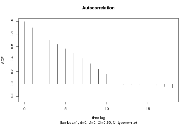
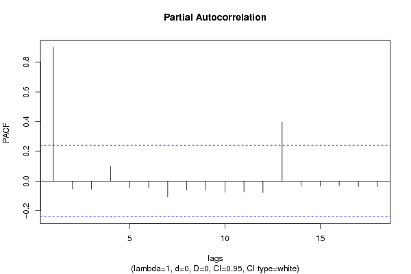
Title produced by software

(Partial) Autocorrelation Function

Date of computation

Fri, 24 Dec 2010 13:35:08 +0000

Cite this page as follows

Statistical Computations at FreeStatistics.org, Office for Research Development and Education, URL https://freestatistics.org/blog/index.php?v=date/2010/Dec/24/t1293197624d43tiwhqusypr28.htm/, Retrieved Tue, 30 Apr 2024 00:12:01 +0000

Statistical Computations at FreeStatistics.org, Office for Research Development and Education, URL https://freestatistics.org/blog/index.php?pk=114933, Retrieved Tue, 30 Apr 2024 00:12:01 +0000

QR Codes:

Paste this QR Code to cite your computation.

Original text written by user:

Prijsverandering in België

IsPrivate?

No (this computation is public)

User-defined keywords

Estimated Impact

144

Family? (F = Feedback message, R = changed R code, M = changed R Module, P = changed Parameters, D = changed Data)

F     [Univariate Data Series] [Airline data] [2007-10-18 09:58:47] [42daae401fd3def69a25014f2252b4c2]
F RMPD  [Cross Correlation Function] [Q7 - zonder trans...] [2008-12-01 20:04:13] [299afd6311e4c20059ea2f05c8dd029d]
F RM D    [Variance Reduction Matrix] [Q8] [2008-12-01 20:20:44] [299afd6311e4c20059ea2f05c8dd029d]
F    D      [Variance Reduction Matrix] [Q8 - 2] [2008-12-01 20:25:07] [299afd6311e4c20059ea2f05c8dd029d]
F RM D        [Standard Deviation-Mean Plot] [Deel 2: Step 1] [2008-12-08 20:09:35] [299afd6311e4c20059ea2f05c8dd029d]
-    D          [Standard Deviation-Mean Plot] [Totale Uitvoer - SMP] [2008-12-17 15:57:12] [299afd6311e4c20059ea2f05c8dd029d]
- RMPD              [(Partial) Autocorrelation Function] [(Partial) Autocor...] [2010-12-24 13:35:08] [fba9c6aa004af59d8497d682e70ddad5] [Current]

Feedback Forum

Post a new message

Dataseries X:

Download CSV

Histogram

Boxplots

3.4
3.4
3.4
-3.5
-3.5
-3.5
-8.3
-8.3
-8.3
-16.7
-16.7
-16.7
-11.6
-11.6
-11.6
-8.4
-8.4
-8.4
-8.6
-8.6
-8.6
0.6
0.6
0.6
-1.5
-1.5
-1.5
9.3
9.3
9.3
2.0
2.0
2.0
-5.5
-5.5
-5.5
4.0
4.0
4.0
-0.5
-0.5
-0.5
10.9
10.9
10.9
19.4
19.4
19.4
13.9
13.9
13.9
10.6
10.6
10.6
4.8
4.8
4.8
4.7
4.7
4.7
-3.9
-3.9
-3.9
-0.2
-0.2
-0.2

Summary of computational transaction
Raw Input	view raw input (R code)
Raw Output	view raw output of R engine
Computing time	2 seconds
R Server	'RServer@AstonUniversity' @ vre.aston.ac.uk

\begin{tabular}{lllllllll}
\hline
Summary of computational transaction \tabularnewline
Raw Input & view raw input (R code)  \tabularnewline
Raw Output & view raw output of R engine  \tabularnewline
Computing time & 2 seconds \tabularnewline
R Server & 'RServer@AstonUniversity' @ vre.aston.ac.uk \tabularnewline
\hline
\end{tabular}
%Source: https://freestatistics.org/blog/index.php?pk=114933&T=0

[TABLE]
[ROW][C]Summary of computational transaction[/C][/ROW]
[ROW][C]Raw Input[/C][C]view raw input (R code) [/C][/ROW]
[ROW][C]Raw Output[/C][C]view raw output of R engine [/C][/ROW]
[ROW][C]Computing time[/C][C]2 seconds[/C][/ROW]
[ROW][C]R Server[/C][C]'RServer@AstonUniversity' @ vre.aston.ac.uk[/C][/ROW]
[/TABLE]
Source: https://freestatistics.org/blog/index.php?pk=114933&T=0

Globally Unique Identifier (entire table): ba.freestatistics.org/blog/index.php?pk=114933&T=0

As an alternative you can also use a QR Code:

The GUIDs for individual cells are displayed in the table below:

Summary of computational transaction
Raw Input	view raw input (R code)
Raw Output	view raw output of R engine
Computing time	2 seconds
R Server	'RServer@AstonUniversity' @ vre.aston.ac.uk

Autocorrelation Function
Time lag k	ACF(k)	T-STAT	P-value
1	0.900885	7.3188	0
2	0.80177	6.5136	0
3	0.702655	5.7084	0
4	0.633076	5.1431	1e-06
5	0.563497	4.5779	1.1e-05
6	0.493918	4.0126	7.8e-05
7	0.409319	3.3253	0.000723
8	0.32472	2.638	0.005195
9	0.240121	1.9507	0.027667
10	0.15739	1.2786	0.102751
11	0.074659	0.6065	0.273121
12	-0.008072	-0.0656	0.473957
13	-0.005892	-0.0479	0.480984
14	-0.003712	-0.0302	0.488017
15	-0.001532	-0.0124	0.495054
16	-0.022348	-0.1816	0.428245
17	-0.043163	-0.3507	0.363481
18	-0.063979	-0.5198	0.302483

\begin{tabular}{lllllllll}
\hline
Autocorrelation Function \tabularnewline
Time lag k & ACF(k) & T-STAT & P-value \tabularnewline
1 & 0.900885 & 7.3188 & 0 \tabularnewline
2 & 0.80177 & 6.5136 & 0 \tabularnewline
3 & 0.702655 & 5.7084 & 0 \tabularnewline
4 & 0.633076 & 5.1431 & 1e-06 \tabularnewline
5 & 0.563497 & 4.5779 & 1.1e-05 \tabularnewline
6 & 0.493918 & 4.0126 & 7.8e-05 \tabularnewline
7 & 0.409319 & 3.3253 & 0.000723 \tabularnewline
8 & 0.32472 & 2.638 & 0.005195 \tabularnewline
9 & 0.240121 & 1.9507 & 0.027667 \tabularnewline
10 & 0.15739 & 1.2786 & 0.102751 \tabularnewline
11 & 0.074659 & 0.6065 & 0.273121 \tabularnewline
12 & -0.008072 & -0.0656 & 0.473957 \tabularnewline
13 & -0.005892 & -0.0479 & 0.480984 \tabularnewline
14 & -0.003712 & -0.0302 & 0.488017 \tabularnewline
15 & -0.001532 & -0.0124 & 0.495054 \tabularnewline
16 & -0.022348 & -0.1816 & 0.428245 \tabularnewline
17 & -0.043163 & -0.3507 & 0.363481 \tabularnewline
18 & -0.063979 & -0.5198 & 0.302483 \tabularnewline
\hline
\end{tabular}
%Source: https://freestatistics.org/blog/index.php?pk=114933&T=1

[TABLE]
[ROW][C]Autocorrelation Function[/C][/ROW]
[ROW][C]Time lag k[/C][C]ACF(k)[/C][C]T-STAT[/C][C]P-value[/C][/ROW]
[ROW][C]1[/C][C]0.900885[/C][C]7.3188[/C][C]0[/C][/ROW]
[ROW][C]2[/C][C]0.80177[/C][C]6.5136[/C][C]0[/C][/ROW]
[ROW][C]3[/C][C]0.702655[/C][C]5.7084[/C][C]0[/C][/ROW]
[ROW][C]4[/C][C]0.633076[/C][C]5.1431[/C][C]1e-06[/C][/ROW]
[ROW][C]5[/C][C]0.563497[/C][C]4.5779[/C][C]1.1e-05[/C][/ROW]
[ROW][C]6[/C][C]0.493918[/C][C]4.0126[/C][C]7.8e-05[/C][/ROW]
[ROW][C]7[/C][C]0.409319[/C][C]3.3253[/C][C]0.000723[/C][/ROW]
[ROW][C]8[/C][C]0.32472[/C][C]2.638[/C][C]0.005195[/C][/ROW]
[ROW][C]9[/C][C]0.240121[/C][C]1.9507[/C][C]0.027667[/C][/ROW]
[ROW][C]10[/C][C]0.15739[/C][C]1.2786[/C][C]0.102751[/C][/ROW]
[ROW][C]11[/C][C]0.074659[/C][C]0.6065[/C][C]0.273121[/C][/ROW]
[ROW][C]12[/C][C]-0.008072[/C][C]-0.0656[/C][C]0.473957[/C][/ROW]
[ROW][C]13[/C][C]-0.005892[/C][C]-0.0479[/C][C]0.480984[/C][/ROW]
[ROW][C]14[/C][C]-0.003712[/C][C]-0.0302[/C][C]0.488017[/C][/ROW]
[ROW][C]15[/C][C]-0.001532[/C][C]-0.0124[/C][C]0.495054[/C][/ROW]
[ROW][C]16[/C][C]-0.022348[/C][C]-0.1816[/C][C]0.428245[/C][/ROW]
[ROW][C]17[/C][C]-0.043163[/C][C]-0.3507[/C][C]0.363481[/C][/ROW]
[ROW][C]18[/C][C]-0.063979[/C][C]-0.5198[/C][C]0.302483[/C][/ROW]
[/TABLE]
Source: https://freestatistics.org/blog/index.php?pk=114933&T=1

Globally Unique Identifier (entire table): ba.freestatistics.org/blog/index.php?pk=114933&T=1

As an alternative you can also use a QR Code:

The GUIDs for individual cells are displayed in the table below:

Autocorrelation Function
Time lag k	ACF(k)	T-STAT	P-value
1	0.900885	7.3188	0
2	0.80177	6.5136	0
3	0.702655	5.7084	0
4	0.633076	5.1431	1e-06
5	0.563497	4.5779	1.1e-05
6	0.493918	4.0126	7.8e-05
7	0.409319	3.3253	0.000723
8	0.32472	2.638	0.005195
9	0.240121	1.9507	0.027667
10	0.15739	1.2786	0.102751
11	0.074659	0.6065	0.273121
12	-0.008072	-0.0656	0.473957
13	-0.005892	-0.0479	0.480984
14	-0.003712	-0.0302	0.488017
15	-0.001532	-0.0124	0.495054
16	-0.022348	-0.1816	0.428245
17	-0.043163	-0.3507	0.363481
18	-0.063979	-0.5198	0.302483

Partial Autocorrelation Function
Time lag k	PACF(k)	T-STAT	P-value
1	0.900885	7.3188	0
2	-0.052141	-0.4236	0.336618
3	-0.05501	-0.4469	0.328205
4	0.099459	0.808	0.210994
5	-0.045057	-0.366	0.357751
6	-0.047183	-0.3833	0.351358
7	-0.107019	-0.8694	0.193883
8	-0.058492	-0.4752	0.318109
9	-0.062126	-0.5047	0.30772
10	-0.076533	-0.6218	0.268121
11	-0.072424	-0.5884	0.279145
12	-0.078079	-0.6343	0.264034
13	0.396571	3.2218	0.00099
14	-0.033736	-0.2741	0.392442
15	-0.034914	-0.2836	0.388786
16	-0.030834	-0.2505	0.401489
17	-0.037136	-0.3017	0.381918
18	-0.038568	-0.3133	0.37751

\begin{tabular}{lllllllll}
\hline
Partial Autocorrelation Function \tabularnewline
Time lag k & PACF(k) & T-STAT & P-value \tabularnewline
1 & 0.900885 & 7.3188 & 0 \tabularnewline
2 & -0.052141 & -0.4236 & 0.336618 \tabularnewline
3 & -0.05501 & -0.4469 & 0.328205 \tabularnewline
4 & 0.099459 & 0.808 & 0.210994 \tabularnewline
5 & -0.045057 & -0.366 & 0.357751 \tabularnewline
6 & -0.047183 & -0.3833 & 0.351358 \tabularnewline
7 & -0.107019 & -0.8694 & 0.193883 \tabularnewline
8 & -0.058492 & -0.4752 & 0.318109 \tabularnewline
9 & -0.062126 & -0.5047 & 0.30772 \tabularnewline
10 & -0.076533 & -0.6218 & 0.268121 \tabularnewline
11 & -0.072424 & -0.5884 & 0.279145 \tabularnewline
12 & -0.078079 & -0.6343 & 0.264034 \tabularnewline
13 & 0.396571 & 3.2218 & 0.00099 \tabularnewline
14 & -0.033736 & -0.2741 & 0.392442 \tabularnewline
15 & -0.034914 & -0.2836 & 0.388786 \tabularnewline
16 & -0.030834 & -0.2505 & 0.401489 \tabularnewline
17 & -0.037136 & -0.3017 & 0.381918 \tabularnewline
18 & -0.038568 & -0.3133 & 0.37751 \tabularnewline
\hline
\end{tabular}
%Source: https://freestatistics.org/blog/index.php?pk=114933&T=2

[TABLE]
[ROW][C]Partial Autocorrelation Function[/C][/ROW]
[ROW][C]Time lag k[/C][C]PACF(k)[/C][C]T-STAT[/C][C]P-value[/C][/ROW]
[ROW][C]1[/C][C]0.900885[/C][C]7.3188[/C][C]0[/C][/ROW]
[ROW][C]2[/C][C]-0.052141[/C][C]-0.4236[/C][C]0.336618[/C][/ROW]
[ROW][C]3[/C][C]-0.05501[/C][C]-0.4469[/C][C]0.328205[/C][/ROW]
[ROW][C]4[/C][C]0.099459[/C][C]0.808[/C][C]0.210994[/C][/ROW]
[ROW][C]5[/C][C]-0.045057[/C][C]-0.366[/C][C]0.357751[/C][/ROW]
[ROW][C]6[/C][C]-0.047183[/C][C]-0.3833[/C][C]0.351358[/C][/ROW]
[ROW][C]7[/C][C]-0.107019[/C][C]-0.8694[/C][C]0.193883[/C][/ROW]
[ROW][C]8[/C][C]-0.058492[/C][C]-0.4752[/C][C]0.318109[/C][/ROW]
[ROW][C]9[/C][C]-0.062126[/C][C]-0.5047[/C][C]0.30772[/C][/ROW]
[ROW][C]10[/C][C]-0.076533[/C][C]-0.6218[/C][C]0.268121[/C][/ROW]
[ROW][C]11[/C][C]-0.072424[/C][C]-0.5884[/C][C]0.279145[/C][/ROW]
[ROW][C]12[/C][C]-0.078079[/C][C]-0.6343[/C][C]0.264034[/C][/ROW]
[ROW][C]13[/C][C]0.396571[/C][C]3.2218[/C][C]0.00099[/C][/ROW]
[ROW][C]14[/C][C]-0.033736[/C][C]-0.2741[/C][C]0.392442[/C][/ROW]
[ROW][C]15[/C][C]-0.034914[/C][C]-0.2836[/C][C]0.388786[/C][/ROW]
[ROW][C]16[/C][C]-0.030834[/C][C]-0.2505[/C][C]0.401489[/C][/ROW]
[ROW][C]17[/C][C]-0.037136[/C][C]-0.3017[/C][C]0.381918[/C][/ROW]
[ROW][C]18[/C][C]-0.038568[/C][C]-0.3133[/C][C]0.37751[/C][/ROW]
[/TABLE]
Source: https://freestatistics.org/blog/index.php?pk=114933&T=2

Globally Unique Identifier (entire table): ba.freestatistics.org/blog/index.php?pk=114933&T=2

As an alternative you can also use a QR Code:

The GUIDs for individual cells are displayed in the table below:

Partial Autocorrelation Function
Time lag k	PACF(k)	T-STAT	P-value
1	0.900885	7.3188	0
2	-0.052141	-0.4236	0.336618
3	-0.05501	-0.4469	0.328205
4	0.099459	0.808	0.210994
5	-0.045057	-0.366	0.357751
6	-0.047183	-0.3833	0.351358
7	-0.107019	-0.8694	0.193883
8	-0.058492	-0.4752	0.318109
9	-0.062126	-0.5047	0.30772
10	-0.076533	-0.6218	0.268121
11	-0.072424	-0.5884	0.279145
12	-0.078079	-0.6343	0.264034
13	0.396571	3.2218	0.00099
14	-0.033736	-0.2741	0.392442
15	-0.034914	-0.2836	0.388786
16	-0.030834	-0.2505	0.401489
17	-0.037136	-0.3017	0.381918
18	-0.038568	-0.3133	0.37751

Figure 1

PNG link

Postscript link

PDF link

Figure 2

PNG link

Postscript link

PDF link

Figure 3

PNG link

Postscript link

PDF link

Parameters (Session):

par1 = Default ; par2 = 1 ; par3 = 0 ; par4 = 0 ; par5 = 12 ; par6 = White Noise ; par7 = 0.95 ;

Parameters (R input):

par1 = Default ; par2 = 1 ; par3 = 0 ; par4 = 0 ; par5 = 12 ; par6 = White Noise ; par7 = 0.95 ; par8 = ;

R code (references can be found in the software module):

if (par1 == 'Default') {
par1 = 10*log10(length(x))
} else {
par1 <- as.numeric(par1)
}
par2 <- as.numeric(par2)
par3 <- as.numeric(par3)
par4 <- as.numeric(par4)
par5 <- as.numeric(par5)
if (par6 == 'White Noise') par6 <- 'white' else par6 <- 'ma'
par7 <- as.numeric(par7)
if (par8 != '') par8 <- as.numeric(par8)
ox <- x
if (par8 == '') {
if (par2 == 0) {
x <- log(x)
} else {
x <- (x ^ par2 - 1) / par2
}
} else {
x <- log(x,base=par8)
}
if (par3 > 0) x <- diff(x,lag=1,difference=par3)
if (par4 > 0) x <- diff(x,lag=par5,difference=par4)
bitmap(file='picts.png')
op <- par(mfrow=c(2,1))
plot(ox,type='l',main='Original Time Series',xlab='time',ylab='value')
if (par8=='') {
mytitle <- paste('Working Time Series (lambda=',par2,', d=',par3,', D=',par4,')',sep='')
mysub <- paste('(lambda=',par2,', d=',par3,', D=',par4,', CI=', par7, ', CI type=',par6,')',sep='')
} else {
mytitle <- paste('Working Time Series (base=',par8,', d=',par3,', D=',par4,')',sep='')
mysub <- paste('(base=',par8,', d=',par3,', D=',par4,', CI=', par7, ', CI type=',par6,')',sep='')
}
plot(x,type='l', main=mytitle,xlab='time',ylab='value')
par(op)
dev.off()
bitmap(file='pic1.png')
racf <- acf(x, par1, main='Autocorrelation', xlab='time lag', ylab='ACF', ci.type=par6, ci=par7, sub=mysub)
dev.off()
bitmap(file='pic2.png')
rpacf <- pacf(x,par1,main='Partial Autocorrelation',xlab='lags',ylab='PACF',sub=mysub)
dev.off()
(myacf <- c(racf$acf))
(mypacf <- c(rpacf$acf))
lengthx <- length(x)
sqrtn <- sqrt(lengthx)
load(file='createtable')
a<-table.start()
a<-table.row.start(a)
a<-table.element(a,'Autocorrelation Function',4,TRUE)
a<-table.row.end(a)
a<-table.row.start(a)
a<-table.element(a,'Time lag k',header=TRUE)
a<-table.element(a,hyperlink('basics.htm','ACF(k)','click here for more information about the Autocorrelation Function'),header=TRUE)
a<-table.element(a,'T-STAT',header=TRUE)
a<-table.element(a,'P-value',header=TRUE)
a<-table.row.end(a)
for (i in 2:(par1+1)) {
a<-table.row.start(a)
a<-table.element(a,i-1,header=TRUE)
a<-table.element(a,round(myacf[i],6))
mytstat <- myacf[i]*sqrtn
a<-table.element(a,round(mytstat,4))
a<-table.element(a,round(1-pt(abs(mytstat),lengthx),6))
a<-table.row.end(a)
}
a<-table.end(a)
table.save(a,file='mytable.tab')
a<-table.start()
a<-table.row.start(a)
a<-table.element(a,'Partial Autocorrelation Function',4,TRUE)
a<-table.row.end(a)
a<-table.row.start(a)
a<-table.element(a,'Time lag k',header=TRUE)
a<-table.element(a,hyperlink('basics.htm','PACF(k)','click here for more information about the Partial Autocorrelation Function'),header=TRUE)
a<-table.element(a,'T-STAT',header=TRUE)
a<-table.element(a,'P-value',header=TRUE)
a<-table.row.end(a)
for (i in 1:par1) {
a<-table.row.start(a)
a<-table.element(a,i,header=TRUE)
a<-table.element(a,round(mypacf[i],6))
mytstat <- mypacf[i]*sqrtn
a<-table.element(a,round(mytstat,4))
a<-table.element(a,round(1-pt(abs(mytstat),lengthx),6))
a<-table.row.end(a)
}
a<-table.end(a)
table.save(a,file='mytable1.tab')

Free Statistics

Description of Statistical Computation

Tree of Dependent Computations

Dataset

Tables (Output of Computation)

Figures (Output of Computation)

Input Parameters & R Code