Free Statistics
of Irreproducible Research!
Description of Statistical Computation | |||||||||||||||||||||||||||||||||||||||||||||||||||||||||||||||||||||||||||||||||||||||||||||||||||||||||||||||||||||||||||||||||||||||||||||||||||||||||||||||||||||||||||||||||||||||||||||||||||||||||||||||||||||||||||||||||||||||||||||||||||||||||||||||||||||||||||||||||||||||||||||||||||||||||||||||||||||||||||||||||||||||||||||||||||||||||||||||||||||||||||||||||||||||||||||||||||||||||||||||||||||||||||||||||||||||||||||||||||||||||||||||||||||||||||||||||||||||||||||||||||||||||||||||||||||||||||||||||||||||||||||||||||||||||||||||||||||||||||||||||||||||||||||||||||||||||||||||||||||||||||||||||||||||||||||||||||||
|---|---|---|---|---|---|---|---|---|---|---|---|---|---|---|---|---|---|---|---|---|---|---|---|---|---|---|---|---|---|---|---|---|---|---|---|---|---|---|---|---|---|---|---|---|---|---|---|---|---|---|---|---|---|---|---|---|---|---|---|---|---|---|---|---|---|---|---|---|---|---|---|---|---|---|---|---|---|---|---|---|---|---|---|---|---|---|---|---|---|---|---|---|---|---|---|---|---|---|---|---|---|---|---|---|---|---|---|---|---|---|---|---|---|---|---|---|---|---|---|---|---|---|---|---|---|---|---|---|---|---|---|---|---|---|---|---|---|---|---|---|---|---|---|---|---|---|---|---|---|---|---|---|---|---|---|---|---|---|---|---|---|---|---|---|---|---|---|---|---|---|---|---|---|---|---|---|---|---|---|---|---|---|---|---|---|---|---|---|---|---|---|---|---|---|---|---|---|---|---|---|---|---|---|---|---|---|---|---|---|---|---|---|---|---|---|---|---|---|---|---|---|---|---|---|---|---|---|---|---|---|---|---|---|---|---|---|---|---|---|---|---|---|---|---|---|---|---|---|---|---|---|---|---|---|---|---|---|---|---|---|---|---|---|---|---|---|---|---|---|---|---|---|---|---|---|---|---|---|---|---|---|---|---|---|---|---|---|---|---|---|---|---|---|---|---|---|---|---|---|---|---|---|---|---|---|---|---|---|---|---|---|---|---|---|---|---|---|---|---|---|---|---|---|---|---|---|---|---|---|---|---|---|---|---|---|---|---|---|---|---|---|---|---|---|---|---|---|---|---|---|---|---|---|---|---|---|---|---|---|---|---|---|---|---|---|---|---|---|---|---|---|---|---|---|---|---|---|---|---|---|---|---|---|---|---|---|---|---|---|---|---|---|---|---|---|---|---|---|---|---|---|---|---|---|---|---|---|---|---|---|---|---|---|---|---|---|---|---|---|---|---|---|---|---|---|---|---|---|---|---|---|---|---|---|---|---|---|---|---|---|---|---|---|---|---|---|---|---|---|---|---|---|---|---|---|---|---|---|---|---|---|---|---|---|---|---|---|---|---|---|---|---|---|---|---|---|---|---|---|---|---|---|---|---|---|---|---|---|---|---|---|---|---|---|---|---|---|---|---|---|---|---|---|---|---|---|---|---|---|---|---|---|---|---|---|---|---|---|---|---|---|---|---|---|---|---|---|---|---|---|---|---|---|---|---|---|---|---|---|---|---|---|---|---|---|---|---|---|---|---|---|---|---|---|---|---|---|---|---|---|---|---|---|---|---|---|---|---|---|---|---|---|---|---|---|---|---|---|---|---|---|---|---|---|---|---|---|---|---|---|---|---|---|---|---|---|---|---|---|---|---|---|---|---|---|---|---|---|---|---|---|---|---|---|---|---|---|---|---|---|---|---|---|---|---|---|---|---|---|
| Author's title | |||||||||||||||||||||||||||||||||||||||||||||||||||||||||||||||||||||||||||||||||||||||||||||||||||||||||||||||||||||||||||||||||||||||||||||||||||||||||||||||||||||||||||||||||||||||||||||||||||||||||||||||||||||||||||||||||||||||||||||||||||||||||||||||||||||||||||||||||||||||||||||||||||||||||||||||||||||||||||||||||||||||||||||||||||||||||||||||||||||||||||||||||||||||||||||||||||||||||||||||||||||||||||||||||||||||||||||||||||||||||||||||||||||||||||||||||||||||||||||||||||||||||||||||||||||||||||||||||||||||||||||||||||||||||||||||||||||||||||||||||||||||||||||||||||||||||||||||||||||||||||||||||||||||||||||||||||||
| Author | *The author of this computation has been verified* | ||||||||||||||||||||||||||||||||||||||||||||||||||||||||||||||||||||||||||||||||||||||||||||||||||||||||||||||||||||||||||||||||||||||||||||||||||||||||||||||||||||||||||||||||||||||||||||||||||||||||||||||||||||||||||||||||||||||||||||||||||||||||||||||||||||||||||||||||||||||||||||||||||||||||||||||||||||||||||||||||||||||||||||||||||||||||||||||||||||||||||||||||||||||||||||||||||||||||||||||||||||||||||||||||||||||||||||||||||||||||||||||||||||||||||||||||||||||||||||||||||||||||||||||||||||||||||||||||||||||||||||||||||||||||||||||||||||||||||||||||||||||||||||||||||||||||||||||||||||||||||||||||||||||||||||||||||||
| R Software Module | rwasp_autocorrelation.wasp | ||||||||||||||||||||||||||||||||||||||||||||||||||||||||||||||||||||||||||||||||||||||||||||||||||||||||||||||||||||||||||||||||||||||||||||||||||||||||||||||||||||||||||||||||||||||||||||||||||||||||||||||||||||||||||||||||||||||||||||||||||||||||||||||||||||||||||||||||||||||||||||||||||||||||||||||||||||||||||||||||||||||||||||||||||||||||||||||||||||||||||||||||||||||||||||||||||||||||||||||||||||||||||||||||||||||||||||||||||||||||||||||||||||||||||||||||||||||||||||||||||||||||||||||||||||||||||||||||||||||||||||||||||||||||||||||||||||||||||||||||||||||||||||||||||||||||||||||||||||||||||||||||||||||||||||||||||||
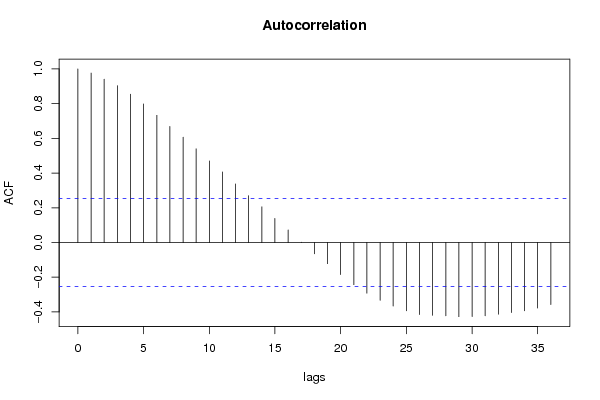
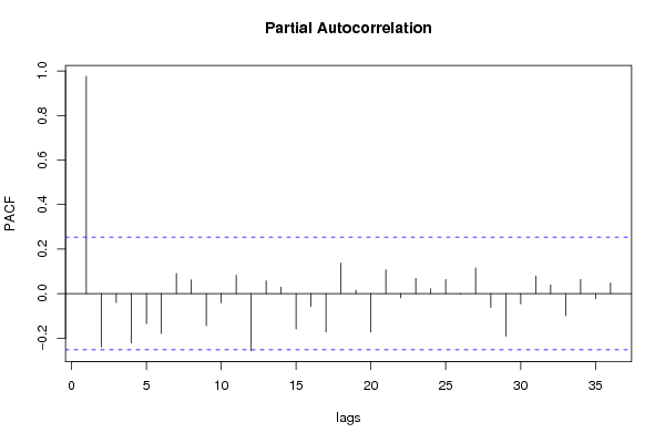
| Title produced by software | (Partial) Autocorrelation Function | ||||||||||||||||||||||||||||||||||||||||||||||||||||||||||||||||||||||||||||||||||||||||||||||||||||||||||||||||||||||||||||||||||||||||||||||||||||||||||||||||||||||||||||||||||||||||||||||||||||||||||||||||||||||||||||||||||||||||||||||||||||||||||||||||||||||||||||||||||||||||||||||||||||||||||||||||||||||||||||||||||||||||||||||||||||||||||||||||||||||||||||||||||||||||||||||||||||||||||||||||||||||||||||||||||||||||||||||||||||||||||||||||||||||||||||||||||||||||||||||||||||||||||||||||||||||||||||||||||||||||||||||||||||||||||||||||||||||||||||||||||||||||||||||||||||||||||||||||||||||||||||||||||||||||||||||||||||
| Date of computation | Fri, 24 Dec 2010 13:07:49 +0000 | ||||||||||||||||||||||||||||||||||||||||||||||||||||||||||||||||||||||||||||||||||||||||||||||||||||||||||||||||||||||||||||||||||||||||||||||||||||||||||||||||||||||||||||||||||||||||||||||||||||||||||||||||||||||||||||||||||||||||||||||||||||||||||||||||||||||||||||||||||||||||||||||||||||||||||||||||||||||||||||||||||||||||||||||||||||||||||||||||||||||||||||||||||||||||||||||||||||||||||||||||||||||||||||||||||||||||||||||||||||||||||||||||||||||||||||||||||||||||||||||||||||||||||||||||||||||||||||||||||||||||||||||||||||||||||||||||||||||||||||||||||||||||||||||||||||||||||||||||||||||||||||||||||||||||||||||||||||
| Cite this page as follows | Statistical Computations at FreeStatistics.org, Office for Research Development and Education, URL https://freestatistics.org/blog/index.php?v=date/2010/Dec/24/t1293195949yupc6zam7v54k0q.htm/, Retrieved Tue, 30 Apr 2024 00:31:56 +0000 | ||||||||||||||||||||||||||||||||||||||||||||||||||||||||||||||||||||||||||||||||||||||||||||||||||||||||||||||||||||||||||||||||||||||||||||||||||||||||||||||||||||||||||||||||||||||||||||||||||||||||||||||||||||||||||||||||||||||||||||||||||||||||||||||||||||||||||||||||||||||||||||||||||||||||||||||||||||||||||||||||||||||||||||||||||||||||||||||||||||||||||||||||||||||||||||||||||||||||||||||||||||||||||||||||||||||||||||||||||||||||||||||||||||||||||||||||||||||||||||||||||||||||||||||||||||||||||||||||||||||||||||||||||||||||||||||||||||||||||||||||||||||||||||||||||||||||||||||||||||||||||||||||||||||||||||||||||||
| Statistical Computations at FreeStatistics.org, Office for Research Development and Education, URL https://freestatistics.org/blog/index.php?pk=114893, Retrieved Tue, 30 Apr 2024 00:31:56 +0000 | |||||||||||||||||||||||||||||||||||||||||||||||||||||||||||||||||||||||||||||||||||||||||||||||||||||||||||||||||||||||||||||||||||||||||||||||||||||||||||||||||||||||||||||||||||||||||||||||||||||||||||||||||||||||||||||||||||||||||||||||||||||||||||||||||||||||||||||||||||||||||||||||||||||||||||||||||||||||||||||||||||||||||||||||||||||||||||||||||||||||||||||||||||||||||||||||||||||||||||||||||||||||||||||||||||||||||||||||||||||||||||||||||||||||||||||||||||||||||||||||||||||||||||||||||||||||||||||||||||||||||||||||||||||||||||||||||||||||||||||||||||||||||||||||||||||||||||||||||||||||||||||||||||||||||||||||||||||
| QR Codes: | |||||||||||||||||||||||||||||||||||||||||||||||||||||||||||||||||||||||||||||||||||||||||||||||||||||||||||||||||||||||||||||||||||||||||||||||||||||||||||||||||||||||||||||||||||||||||||||||||||||||||||||||||||||||||||||||||||||||||||||||||||||||||||||||||||||||||||||||||||||||||||||||||||||||||||||||||||||||||||||||||||||||||||||||||||||||||||||||||||||||||||||||||||||||||||||||||||||||||||||||||||||||||||||||||||||||||||||||||||||||||||||||||||||||||||||||||||||||||||||||||||||||||||||||||||||||||||||||||||||||||||||||||||||||||||||||||||||||||||||||||||||||||||||||||||||||||||||||||||||||||||||||||||||||||||||||||||||
|
| |||||||||||||||||||||||||||||||||||||||||||||||||||||||||||||||||||||||||||||||||||||||||||||||||||||||||||||||||||||||||||||||||||||||||||||||||||||||||||||||||||||||||||||||||||||||||||||||||||||||||||||||||||||||||||||||||||||||||||||||||||||||||||||||||||||||||||||||||||||||||||||||||||||||||||||||||||||||||||||||||||||||||||||||||||||||||||||||||||||||||||||||||||||||||||||||||||||||||||||||||||||||||||||||||||||||||||||||||||||||||||||||||||||||||||||||||||||||||||||||||||||||||||||||||||||||||||||||||||||||||||||||||||||||||||||||||||||||||||||||||||||||||||||||||||||||||||||||||||||||||||||||||||||||||||||||||||||
| Original text written by user: | |||||||||||||||||||||||||||||||||||||||||||||||||||||||||||||||||||||||||||||||||||||||||||||||||||||||||||||||||||||||||||||||||||||||||||||||||||||||||||||||||||||||||||||||||||||||||||||||||||||||||||||||||||||||||||||||||||||||||||||||||||||||||||||||||||||||||||||||||||||||||||||||||||||||||||||||||||||||||||||||||||||||||||||||||||||||||||||||||||||||||||||||||||||||||||||||||||||||||||||||||||||||||||||||||||||||||||||||||||||||||||||||||||||||||||||||||||||||||||||||||||||||||||||||||||||||||||||||||||||||||||||||||||||||||||||||||||||||||||||||||||||||||||||||||||||||||||||||||||||||||||||||||||||||||||||||||||||
| IsPrivate? | No (this computation is public) | ||||||||||||||||||||||||||||||||||||||||||||||||||||||||||||||||||||||||||||||||||||||||||||||||||||||||||||||||||||||||||||||||||||||||||||||||||||||||||||||||||||||||||||||||||||||||||||||||||||||||||||||||||||||||||||||||||||||||||||||||||||||||||||||||||||||||||||||||||||||||||||||||||||||||||||||||||||||||||||||||||||||||||||||||||||||||||||||||||||||||||||||||||||||||||||||||||||||||||||||||||||||||||||||||||||||||||||||||||||||||||||||||||||||||||||||||||||||||||||||||||||||||||||||||||||||||||||||||||||||||||||||||||||||||||||||||||||||||||||||||||||||||||||||||||||||||||||||||||||||||||||||||||||||||||||||||||||
| User-defined keywords | |||||||||||||||||||||||||||||||||||||||||||||||||||||||||||||||||||||||||||||||||||||||||||||||||||||||||||||||||||||||||||||||||||||||||||||||||||||||||||||||||||||||||||||||||||||||||||||||||||||||||||||||||||||||||||||||||||||||||||||||||||||||||||||||||||||||||||||||||||||||||||||||||||||||||||||||||||||||||||||||||||||||||||||||||||||||||||||||||||||||||||||||||||||||||||||||||||||||||||||||||||||||||||||||||||||||||||||||||||||||||||||||||||||||||||||||||||||||||||||||||||||||||||||||||||||||||||||||||||||||||||||||||||||||||||||||||||||||||||||||||||||||||||||||||||||||||||||||||||||||||||||||||||||||||||||||||||||
| Estimated Impact | 129 | ||||||||||||||||||||||||||||||||||||||||||||||||||||||||||||||||||||||||||||||||||||||||||||||||||||||||||||||||||||||||||||||||||||||||||||||||||||||||||||||||||||||||||||||||||||||||||||||||||||||||||||||||||||||||||||||||||||||||||||||||||||||||||||||||||||||||||||||||||||||||||||||||||||||||||||||||||||||||||||||||||||||||||||||||||||||||||||||||||||||||||||||||||||||||||||||||||||||||||||||||||||||||||||||||||||||||||||||||||||||||||||||||||||||||||||||||||||||||||||||||||||||||||||||||||||||||||||||||||||||||||||||||||||||||||||||||||||||||||||||||||||||||||||||||||||||||||||||||||||||||||||||||||||||||||||||||||||
Tree of Dependent Computations | |||||||||||||||||||||||||||||||||||||||||||||||||||||||||||||||||||||||||||||||||||||||||||||||||||||||||||||||||||||||||||||||||||||||||||||||||||||||||||||||||||||||||||||||||||||||||||||||||||||||||||||||||||||||||||||||||||||||||||||||||||||||||||||||||||||||||||||||||||||||||||||||||||||||||||||||||||||||||||||||||||||||||||||||||||||||||||||||||||||||||||||||||||||||||||||||||||||||||||||||||||||||||||||||||||||||||||||||||||||||||||||||||||||||||||||||||||||||||||||||||||||||||||||||||||||||||||||||||||||||||||||||||||||||||||||||||||||||||||||||||||||||||||||||||||||||||||||||||||||||||||||||||||||||||||||||||||||
| Family? (F = Feedback message, R = changed R code, M = changed R Module, P = changed Parameters, D = changed Data) | |||||||||||||||||||||||||||||||||||||||||||||||||||||||||||||||||||||||||||||||||||||||||||||||||||||||||||||||||||||||||||||||||||||||||||||||||||||||||||||||||||||||||||||||||||||||||||||||||||||||||||||||||||||||||||||||||||||||||||||||||||||||||||||||||||||||||||||||||||||||||||||||||||||||||||||||||||||||||||||||||||||||||||||||||||||||||||||||||||||||||||||||||||||||||||||||||||||||||||||||||||||||||||||||||||||||||||||||||||||||||||||||||||||||||||||||||||||||||||||||||||||||||||||||||||||||||||||||||||||||||||||||||||||||||||||||||||||||||||||||||||||||||||||||||||||||||||||||||||||||||||||||||||||||||||||||||||||
| - [(Partial) Autocorrelation Function] [autocorrelatie bel20] [2008-12-10 18:48:27] [74be16979710d4c4e7c6647856088456] - MPD [(Partial) Autocorrelation Function] [] [2009-12-15 15:19:26] [2f674a53c3d7aaa1bcf80e66074d3c9b] - PD [(Partial) Autocorrelation Function] [paper] [2010-12-24 13:07:49] [5d6b44265a1bea1cb58a5907cde468a5] [Current] | |||||||||||||||||||||||||||||||||||||||||||||||||||||||||||||||||||||||||||||||||||||||||||||||||||||||||||||||||||||||||||||||||||||||||||||||||||||||||||||||||||||||||||||||||||||||||||||||||||||||||||||||||||||||||||||||||||||||||||||||||||||||||||||||||||||||||||||||||||||||||||||||||||||||||||||||||||||||||||||||||||||||||||||||||||||||||||||||||||||||||||||||||||||||||||||||||||||||||||||||||||||||||||||||||||||||||||||||||||||||||||||||||||||||||||||||||||||||||||||||||||||||||||||||||||||||||||||||||||||||||||||||||||||||||||||||||||||||||||||||||||||||||||||||||||||||||||||||||||||||||||||||||||||||||||||||||||||
| Feedback Forum | |||||||||||||||||||||||||||||||||||||||||||||||||||||||||||||||||||||||||||||||||||||||||||||||||||||||||||||||||||||||||||||||||||||||||||||||||||||||||||||||||||||||||||||||||||||||||||||||||||||||||||||||||||||||||||||||||||||||||||||||||||||||||||||||||||||||||||||||||||||||||||||||||||||||||||||||||||||||||||||||||||||||||||||||||||||||||||||||||||||||||||||||||||||||||||||||||||||||||||||||||||||||||||||||||||||||||||||||||||||||||||||||||||||||||||||||||||||||||||||||||||||||||||||||||||||||||||||||||||||||||||||||||||||||||||||||||||||||||||||||||||||||||||||||||||||||||||||||||||||||||||||||||||||||||||||||||||||
Post a new message | |||||||||||||||||||||||||||||||||||||||||||||||||||||||||||||||||||||||||||||||||||||||||||||||||||||||||||||||||||||||||||||||||||||||||||||||||||||||||||||||||||||||||||||||||||||||||||||||||||||||||||||||||||||||||||||||||||||||||||||||||||||||||||||||||||||||||||||||||||||||||||||||||||||||||||||||||||||||||||||||||||||||||||||||||||||||||||||||||||||||||||||||||||||||||||||||||||||||||||||||||||||||||||||||||||||||||||||||||||||||||||||||||||||||||||||||||||||||||||||||||||||||||||||||||||||||||||||||||||||||||||||||||||||||||||||||||||||||||||||||||||||||||||||||||||||||||||||||||||||||||||||||||||||||||||||||||||||
Dataset | |||||||||||||||||||||||||||||||||||||||||||||||||||||||||||||||||||||||||||||||||||||||||||||||||||||||||||||||||||||||||||||||||||||||||||||||||||||||||||||||||||||||||||||||||||||||||||||||||||||||||||||||||||||||||||||||||||||||||||||||||||||||||||||||||||||||||||||||||||||||||||||||||||||||||||||||||||||||||||||||||||||||||||||||||||||||||||||||||||||||||||||||||||||||||||||||||||||||||||||||||||||||||||||||||||||||||||||||||||||||||||||||||||||||||||||||||||||||||||||||||||||||||||||||||||||||||||||||||||||||||||||||||||||||||||||||||||||||||||||||||||||||||||||||||||||||||||||||||||||||||||||||||||||||||||||||||||||
| Dataseries X: | |||||||||||||||||||||||||||||||||||||||||||||||||||||||||||||||||||||||||||||||||||||||||||||||||||||||||||||||||||||||||||||||||||||||||||||||||||||||||||||||||||||||||||||||||||||||||||||||||||||||||||||||||||||||||||||||||||||||||||||||||||||||||||||||||||||||||||||||||||||||||||||||||||||||||||||||||||||||||||||||||||||||||||||||||||||||||||||||||||||||||||||||||||||||||||||||||||||||||||||||||||||||||||||||||||||||||||||||||||||||||||||||||||||||||||||||||||||||||||||||||||||||||||||||||||||||||||||||||||||||||||||||||||||||||||||||||||||||||||||||||||||||||||||||||||||||||||||||||||||||||||||||||||||||||||||||||||||
3494,17 3667,03 3813,06 3917,96 3895,51 3801,06 3570,12 3701,61 3862,27 3970,1 4138,52 4199,75 4290,89 4443,91 4502,64 4356,98 4591,27 4696,96 4621,4 4562,84 4202,52 4296,49 4435,23 4105,18 4116,68 3844,49 3720,98 3674,4 3857,62 3801,06 3504,37 3032,6 3047,03 2962,34 2197,82 2014,45 1862,83 1905,41 1810,99 1670,07 1864,44 2052,02 2029,6 2070,83 2293,41 2443,27 2513,17 2466,92 2502,66 2539,91 2482,6 2626,15 2656,32 2446,66 2467,38 2462,32 2504,58 2579,39 2649,24 2636,87 | |||||||||||||||||||||||||||||||||||||||||||||||||||||||||||||||||||||||||||||||||||||||||||||||||||||||||||||||||||||||||||||||||||||||||||||||||||||||||||||||||||||||||||||||||||||||||||||||||||||||||||||||||||||||||||||||||||||||||||||||||||||||||||||||||||||||||||||||||||||||||||||||||||||||||||||||||||||||||||||||||||||||||||||||||||||||||||||||||||||||||||||||||||||||||||||||||||||||||||||||||||||||||||||||||||||||||||||||||||||||||||||||||||||||||||||||||||||||||||||||||||||||||||||||||||||||||||||||||||||||||||||||||||||||||||||||||||||||||||||||||||||||||||||||||||||||||||||||||||||||||||||||||||||||||||||||||||||
Tables (Output of Computation) | |||||||||||||||||||||||||||||||||||||||||||||||||||||||||||||||||||||||||||||||||||||||||||||||||||||||||||||||||||||||||||||||||||||||||||||||||||||||||||||||||||||||||||||||||||||||||||||||||||||||||||||||||||||||||||||||||||||||||||||||||||||||||||||||||||||||||||||||||||||||||||||||||||||||||||||||||||||||||||||||||||||||||||||||||||||||||||||||||||||||||||||||||||||||||||||||||||||||||||||||||||||||||||||||||||||||||||||||||||||||||||||||||||||||||||||||||||||||||||||||||||||||||||||||||||||||||||||||||||||||||||||||||||||||||||||||||||||||||||||||||||||||||||||||||||||||||||||||||||||||||||||||||||||||||||||||||||||
| |||||||||||||||||||||||||||||||||||||||||||||||||||||||||||||||||||||||||||||||||||||||||||||||||||||||||||||||||||||||||||||||||||||||||||||||||||||||||||||||||||||||||||||||||||||||||||||||||||||||||||||||||||||||||||||||||||||||||||||||||||||||||||||||||||||||||||||||||||||||||||||||||||||||||||||||||||||||||||||||||||||||||||||||||||||||||||||||||||||||||||||||||||||||||||||||||||||||||||||||||||||||||||||||||||||||||||||||||||||||||||||||||||||||||||||||||||||||||||||||||||||||||||||||||||||||||||||||||||||||||||||||||||||||||||||||||||||||||||||||||||||||||||||||||||||||||||||||||||||||||||||||||||||||||||||||||||||
Figures (Output of Computation) | |||||||||||||||||||||||||||||||||||||||||||||||||||||||||||||||||||||||||||||||||||||||||||||||||||||||||||||||||||||||||||||||||||||||||||||||||||||||||||||||||||||||||||||||||||||||||||||||||||||||||||||||||||||||||||||||||||||||||||||||||||||||||||||||||||||||||||||||||||||||||||||||||||||||||||||||||||||||||||||||||||||||||||||||||||||||||||||||||||||||||||||||||||||||||||||||||||||||||||||||||||||||||||||||||||||||||||||||||||||||||||||||||||||||||||||||||||||||||||||||||||||||||||||||||||||||||||||||||||||||||||||||||||||||||||||||||||||||||||||||||||||||||||||||||||||||||||||||||||||||||||||||||||||||||||||||||||||
Input Parameters & R Code | |||||||||||||||||||||||||||||||||||||||||||||||||||||||||||||||||||||||||||||||||||||||||||||||||||||||||||||||||||||||||||||||||||||||||||||||||||||||||||||||||||||||||||||||||||||||||||||||||||||||||||||||||||||||||||||||||||||||||||||||||||||||||||||||||||||||||||||||||||||||||||||||||||||||||||||||||||||||||||||||||||||||||||||||||||||||||||||||||||||||||||||||||||||||||||||||||||||||||||||||||||||||||||||||||||||||||||||||||||||||||||||||||||||||||||||||||||||||||||||||||||||||||||||||||||||||||||||||||||||||||||||||||||||||||||||||||||||||||||||||||||||||||||||||||||||||||||||||||||||||||||||||||||||||||||||||||||||
| Parameters (Session): | |||||||||||||||||||||||||||||||||||||||||||||||||||||||||||||||||||||||||||||||||||||||||||||||||||||||||||||||||||||||||||||||||||||||||||||||||||||||||||||||||||||||||||||||||||||||||||||||||||||||||||||||||||||||||||||||||||||||||||||||||||||||||||||||||||||||||||||||||||||||||||||||||||||||||||||||||||||||||||||||||||||||||||||||||||||||||||||||||||||||||||||||||||||||||||||||||||||||||||||||||||||||||||||||||||||||||||||||||||||||||||||||||||||||||||||||||||||||||||||||||||||||||||||||||||||||||||||||||||||||||||||||||||||||||||||||||||||||||||||||||||||||||||||||||||||||||||||||||||||||||||||||||||||||||||||||||||||
| par1 = 36 ; par2 = 1 ; par3 = 0 ; par4 = 0 ; par5 = 12 ; par6 = MA ; | |||||||||||||||||||||||||||||||||||||||||||||||||||||||||||||||||||||||||||||||||||||||||||||||||||||||||||||||||||||||||||||||||||||||||||||||||||||||||||||||||||||||||||||||||||||||||||||||||||||||||||||||||||||||||||||||||||||||||||||||||||||||||||||||||||||||||||||||||||||||||||||||||||||||||||||||||||||||||||||||||||||||||||||||||||||||||||||||||||||||||||||||||||||||||||||||||||||||||||||||||||||||||||||||||||||||||||||||||||||||||||||||||||||||||||||||||||||||||||||||||||||||||||||||||||||||||||||||||||||||||||||||||||||||||||||||||||||||||||||||||||||||||||||||||||||||||||||||||||||||||||||||||||||||||||||||||||||
| Parameters (R input): | |||||||||||||||||||||||||||||||||||||||||||||||||||||||||||||||||||||||||||||||||||||||||||||||||||||||||||||||||||||||||||||||||||||||||||||||||||||||||||||||||||||||||||||||||||||||||||||||||||||||||||||||||||||||||||||||||||||||||||||||||||||||||||||||||||||||||||||||||||||||||||||||||||||||||||||||||||||||||||||||||||||||||||||||||||||||||||||||||||||||||||||||||||||||||||||||||||||||||||||||||||||||||||||||||||||||||||||||||||||||||||||||||||||||||||||||||||||||||||||||||||||||||||||||||||||||||||||||||||||||||||||||||||||||||||||||||||||||||||||||||||||||||||||||||||||||||||||||||||||||||||||||||||||||||||||||||||||
| par1 = 36 ; par2 = 1 ; par3 = 0 ; par4 = 0 ; par5 = 12 ; par6 = MA ; par7 = ; par8 = ; | |||||||||||||||||||||||||||||||||||||||||||||||||||||||||||||||||||||||||||||||||||||||||||||||||||||||||||||||||||||||||||||||||||||||||||||||||||||||||||||||||||||||||||||||||||||||||||||||||||||||||||||||||||||||||||||||||||||||||||||||||||||||||||||||||||||||||||||||||||||||||||||||||||||||||||||||||||||||||||||||||||||||||||||||||||||||||||||||||||||||||||||||||||||||||||||||||||||||||||||||||||||||||||||||||||||||||||||||||||||||||||||||||||||||||||||||||||||||||||||||||||||||||||||||||||||||||||||||||||||||||||||||||||||||||||||||||||||||||||||||||||||||||||||||||||||||||||||||||||||||||||||||||||||||||||||||||||||
| R code (references can be found in the software module): | |||||||||||||||||||||||||||||||||||||||||||||||||||||||||||||||||||||||||||||||||||||||||||||||||||||||||||||||||||||||||||||||||||||||||||||||||||||||||||||||||||||||||||||||||||||||||||||||||||||||||||||||||||||||||||||||||||||||||||||||||||||||||||||||||||||||||||||||||||||||||||||||||||||||||||||||||||||||||||||||||||||||||||||||||||||||||||||||||||||||||||||||||||||||||||||||||||||||||||||||||||||||||||||||||||||||||||||||||||||||||||||||||||||||||||||||||||||||||||||||||||||||||||||||||||||||||||||||||||||||||||||||||||||||||||||||||||||||||||||||||||||||||||||||||||||||||||||||||||||||||||||||||||||||||||||||||||||
if (par1 == 'Default') { | |||||||||||||||||||||||||||||||||||||||||||||||||||||||||||||||||||||||||||||||||||||||||||||||||||||||||||||||||||||||||||||||||||||||||||||||||||||||||||||||||||||||||||||||||||||||||||||||||||||||||||||||||||||||||||||||||||||||||||||||||||||||||||||||||||||||||||||||||||||||||||||||||||||||||||||||||||||||||||||||||||||||||||||||||||||||||||||||||||||||||||||||||||||||||||||||||||||||||||||||||||||||||||||||||||||||||||||||||||||||||||||||||||||||||||||||||||||||||||||||||||||||||||||||||||||||||||||||||||||||||||||||||||||||||||||||||||||||||||||||||||||||||||||||||||||||||||||||||||||||||||||||||||||||||||||||||||||