Repository of Reproducible Computations

Free Statistics

of Irreproducible Research!

Author's title

Author

*The author of this computation has been verified*

R Software Module

rwasp_edauni.wasp

Title produced by software

Univariate Explorative Data Analysis

Date of computation

Fri, 24 Dec 2010 12:49:48 +0000

Cite this page as follows

Statistical Computations at FreeStatistics.org, Office for Research Development and Education, URL https://freestatistics.org/blog/index.php?v=date/2010/Dec/24/t1293194872n33yobwdlxdpjv0.htm/, Retrieved Tue, 30 Apr 2024 03:57:34 +0000

Statistical Computations at FreeStatistics.org, Office for Research Development and Education, URL https://freestatistics.org/blog/index.php?pk=114880, Retrieved Tue, 30 Apr 2024 03:57:34 +0000

QR Codes:

Paste this QR Code to cite your computation.

Original text written by user:

IsPrivate?

No (this computation is public)

User-defined keywords

Estimated Impact

126

Family? (F = Feedback message, R = changed R code, M = changed R Module, P = changed Parameters, D = changed Data)

-     [Univariate Explorative Data Analysis] [paper] [2007-12-11 21:01:08] [b3bb3ec527e23fa7d74d4348b38c8499]
- RMPD  [Univariate Explorative Data Analysis] [PAPER] [2009-12-30 15:50:30] [23722951c28e05bb35cc9a97084fe0d9]
-   PD    [Univariate Explorative Data Analysis] [Univariate EDA pa...] [2010-12-17 15:14:41] [b659239b537e56f17142ee5c56ad6265]
-   PD        [Univariate Explorative Data Analysis] [Run sequence plot...] [2010-12-24 12:49:48] [efffa7146cfe4c2b113f6c7f36d84ca0] [Current]

Feedback Forum

Post a new message

Dataseries X:

Download CSV

Histogram

Boxplots

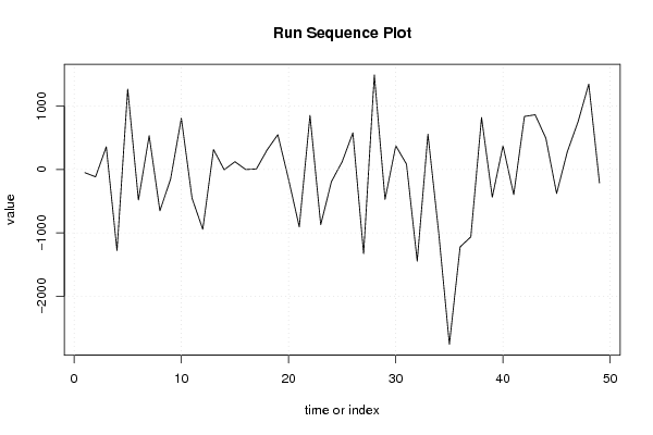
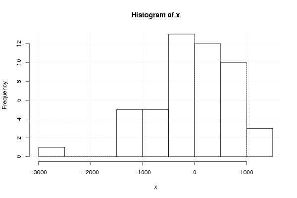
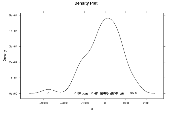
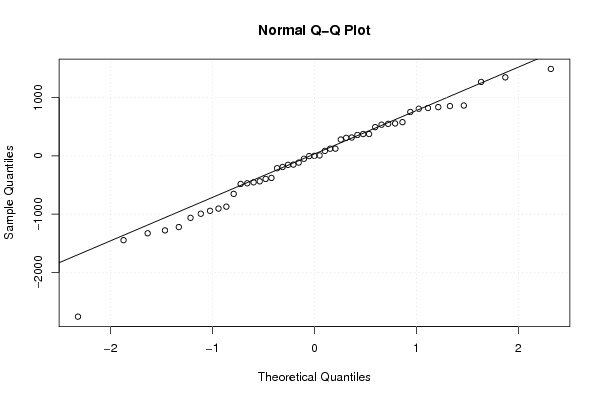
-49.7893339813624
-115.855857347157
358.642252325575
-1280.23404859543
1269.7990218444
-482.344439925045
535.432156472485
-653.350665670356
-150.255607623481
809.700340422624
-454.25759298969
-944.643265379427
315.20994572738
-4.19622349469063
122.766997172271
0.263819130037385
7.82728106033063
309.789819115024
550.179633243721
-154.686633687727
-905.855795506139
855.608436659643
-873.24999022707
-190.895544647361
123.512252726179
579.148230586512
-1330.15873241708
1493.42083518269
-471.236978042281
375.446281752056
84.7030430928148
-1448.7429878622
556.696970316013
-994.720490616971
-2762.85125636168
-1223.45771147529
-1064.55765279704
821.83469984857
-437.67345344376
375.180756215468
-396.843780362746
837.847042453338
864.953789085965
493.563033484152
-378.994495101279
280.453936285203
754.180578928203
1349.24340665111
-212.749295852145

Summary of computational transaction
Raw Input	view raw input (R code)
Raw Output	view raw output of R engine
Computing time	2 seconds
R Server	'Sir Ronald Aylmer Fisher' @ 193.190.124.24

\begin{tabular}{lllllllll}
\hline
Summary of computational transaction \tabularnewline
Raw Input & view raw input (R code)  \tabularnewline
Raw Output & view raw output of R engine  \tabularnewline
Computing time & 2 seconds \tabularnewline
R Server & 'Sir Ronald Aylmer Fisher' @ 193.190.124.24 \tabularnewline
\hline
\end{tabular}
%Source: https://freestatistics.org/blog/index.php?pk=114880&T=0

[TABLE]
[ROW][C]Summary of computational transaction[/C][/ROW]
[ROW][C]Raw Input[/C][C]view raw input (R code) [/C][/ROW]
[ROW][C]Raw Output[/C][C]view raw output of R engine [/C][/ROW]
[ROW][C]Computing time[/C][C]2 seconds[/C][/ROW]
[ROW][C]R Server[/C][C]'Sir Ronald Aylmer Fisher' @ 193.190.124.24[/C][/ROW]
[/TABLE]
Source: https://freestatistics.org/blog/index.php?pk=114880&T=0

Globally Unique Identifier (entire table): ba.freestatistics.org/blog/index.php?pk=114880&T=0

As an alternative you can also use a QR Code:

The GUIDs for individual cells are displayed in the table below:

Summary of computational transaction
Raw Input	view raw input (R code)
Raw Output	view raw output of R engine
Computing time	2 seconds
R Server	'Sir Ronald Aylmer Fisher' @ 193.190.124.24

Descriptive Statistics
# observations	49
minimum	-2762.85125636168
Q1	-471.236978042281
median	0.263819130037385
mean	-58.2897402780744
Q3	535.432156472485
maximum	1493.42083518269

\begin{tabular}{lllllllll}
\hline
Descriptive Statistics \tabularnewline
# observations & 49 \tabularnewline
minimum & -2762.85125636168 \tabularnewline
Q1 & -471.236978042281 \tabularnewline
median & 0.263819130037385 \tabularnewline
mean & -58.2897402780744 \tabularnewline
Q3 & 535.432156472485 \tabularnewline
maximum & 1493.42083518269 \tabularnewline
\hline
\end{tabular}
%Source: https://freestatistics.org/blog/index.php?pk=114880&T=1

[TABLE]
[ROW][C]Descriptive Statistics[/C][/ROW]
[ROW][C]# observations[/C][C]49[/C][/ROW]
[ROW][C]minimum[/C][C]-2762.85125636168[/C][/ROW]
[ROW][C]Q1[/C][C]-471.236978042281[/C][/ROW]
[ROW][C]median[/C][C]0.263819130037385[/C][/ROW]
[ROW][C]mean[/C][C]-58.2897402780744[/C][/ROW]
[ROW][C]Q3[/C][C]535.432156472485[/C][/ROW]
[ROW][C]maximum[/C][C]1493.42083518269[/C][/ROW]
[/TABLE]
Source: https://freestatistics.org/blog/index.php?pk=114880&T=1

Globally Unique Identifier (entire table): ba.freestatistics.org/blog/index.php?pk=114880&T=1

As an alternative you can also use a QR Code:

The GUIDs for individual cells are displayed in the table below:

Descriptive Statistics
# observations	49
minimum	-2762.85125636168
Q1	-471.236978042281
median	0.263819130037385
mean	-58.2897402780744
Q3	535.432156472485
maximum	1493.42083518269

Figure 1

PNG link

Postscript link

PDF link

Figure 2

PNG link

Postscript link

PDF link

Figure 3

PNG link

Postscript link

PDF link

Figure 4

PNG link

Postscript link

PDF link

Figure 5

PNG link

Postscript link

PDF link

Figure 6

PNG link

Postscript link

PDF link

Figure 7

PNG link

Postscript link

PDF link

Parameters (Session):

par1 = 0 ; par2 = 0 ;

Parameters (R input):

par1 = 0 ; par2 = 0 ;

R code (references can be found in the software module):

par1 <- as.numeric(par1)
par2 <- as.numeric(par2)
x <- as.ts(x)
library(lattice)
bitmap(file='pic1.png')
plot(x,type='l',main='Run Sequence Plot',xlab='time or index',ylab='value')
grid()
dev.off()
bitmap(file='pic2.png')
hist(x)
grid()
dev.off()
bitmap(file='pic3.png')
if (par1 > 0)
{
densityplot(~x,col='black',main=paste('Density Plot   bw = ',par1),bw=par1)
} else {
densityplot(~x,col='black',main='Density Plot')
}
dev.off()
bitmap(file='pic4.png')
qqnorm(x)
qqline(x)
grid()
dev.off()
if (par2 > 0)
{
bitmap(file='lagplot1.png')
dum <- cbind(lag(x,k=1),x)
dum
dum1 <- dum[2:length(x),]
dum1
z <- as.data.frame(dum1)
z
plot(z,main='Lag plot (k=1), lowess, and regression line')
lines(lowess(z))
abline(lm(z))
dev.off()
if (par2 > 1) {
bitmap(file='lagplotpar2.png')
dum <- cbind(lag(x,k=par2),x)
dum
dum1 <- dum[(par2+1):length(x),]
dum1
z <- as.data.frame(dum1)
z
mylagtitle <- 'Lag plot (k='
mylagtitle <- paste(mylagtitle,par2,sep='')
mylagtitle <- paste(mylagtitle,'), and lowess',sep='')
plot(z,main=mylagtitle)
lines(lowess(z))
dev.off()
}
bitmap(file='pic5.png')
acf(x,lag.max=par2,main='Autocorrelation Function')
grid()
dev.off()
}
summary(x)
load(file='createtable')
a<-table.start()
a<-table.row.start(a)
a<-table.element(a,'Descriptive Statistics',2,TRUE)
a<-table.row.end(a)
a<-table.row.start(a)
a<-table.element(a,'# observations',header=TRUE)
a<-table.element(a,length(x))
a<-table.row.end(a)
a<-table.row.start(a)
a<-table.element(a,'minimum',header=TRUE)
a<-table.element(a,min(x))
a<-table.row.end(a)
a<-table.row.start(a)
a<-table.element(a,'Q1',header=TRUE)
a<-table.element(a,quantile(x,0.25))
a<-table.row.end(a)
a<-table.row.start(a)
a<-table.element(a,'median',header=TRUE)
a<-table.element(a,median(x))
a<-table.row.end(a)
a<-table.row.start(a)
a<-table.element(a,'mean',header=TRUE)
a<-table.element(a,mean(x))
a<-table.row.end(a)
a<-table.row.start(a)
a<-table.element(a,'Q3',header=TRUE)
a<-table.element(a,quantile(x,0.75))
a<-table.row.end(a)
a<-table.row.start(a)
a<-table.element(a,'maximum',header=TRUE)
a<-table.element(a,max(x))
a<-table.row.end(a)
a<-table.end(a)
table.save(a,file='mytable.tab')

Free Statistics

Description of Statistical Computation

Tree of Dependent Computations

Dataset

Tables (Output of Computation)

Figures (Output of Computation)

Input Parameters & R Code