Repository of Reproducible Computations

Free Statistics

of Irreproducible Research!

Author's title

Author

*The author of this computation has been verified*

R Software Module

rwasp_autocorrelation.wasp

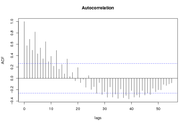
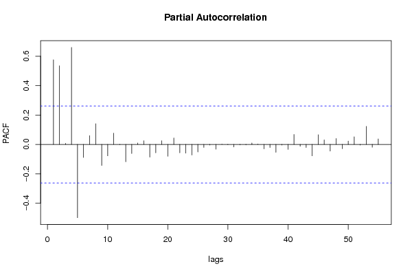
Title produced by software

(Partial) Autocorrelation Function

Date of computation

Fri, 24 Dec 2010 12:03:15 +0000

Cite this page as follows

Statistical Computations at FreeStatistics.org, Office for Research Development and Education, URL https://freestatistics.org/blog/index.php?v=date/2010/Dec/24/t1293192076gdw9urkll6nfgp0.htm/, Retrieved Tue, 30 Apr 2024 03:53:14 +0000

Statistical Computations at FreeStatistics.org, Office for Research Development and Education, URL https://freestatistics.org/blog/index.php?pk=114800, Retrieved Tue, 30 Apr 2024 03:53:14 +0000

QR Codes:

Paste this QR Code to cite your computation.

Original text written by user:

IsPrivate?

No (this computation is public)

User-defined keywords

Estimated Impact

159

Family? (F = Feedback message, R = changed R code, M = changed R Module, P = changed Parameters, D = changed Data)

-     [Standard Deviation-Mean Plot] [SMP prof bach] [2008-12-15 22:25:20] [bc937651ef42bf891200cf0e0edc7238]
- RM    [Variance Reduction Matrix] [VRM prof bach] [2008-12-15 22:31:00] [bc937651ef42bf891200cf0e0edc7238]
- RMP     [(Partial) Autocorrelation Function] [ARIMA Prof bach A...] [2008-12-15 22:38:57] [bc937651ef42bf891200cf0e0edc7238]
-   P       [(Partial) Autocorrelation Function] [ARIMA ACF prof ba...] [2008-12-15 22:41:53] [bc937651ef42bf891200cf0e0edc7238]
-   P         [(Partial) Autocorrelation Function] [acf prof bach L =...] [2008-12-19 15:35:04] [bc937651ef42bf891200cf0e0edc7238]
-  MPD            [(Partial) Autocorrelation Function] [] [2010-12-24 12:03:15] [b91d9cfbf8712a09013bf3c2e3081c55] [Current]

Feedback Forum

Post a new message

Dataseries X:

Download CSV

Histogram

Boxplots

Summary of computational transaction
Raw Input	view raw input (R code)
Raw Output	view raw output of R engine
Computing time	2 seconds
R Server	'RServer@AstonUniversity' @ vre.aston.ac.uk

\begin{tabular}{lllllllll}
\hline
Summary of computational transaction \tabularnewline
Raw Input & view raw input (R code)  \tabularnewline
Raw Output & view raw output of R engine  \tabularnewline
Computing time & 2 seconds \tabularnewline
R Server & 'RServer@AstonUniversity' @ vre.aston.ac.uk \tabularnewline
\hline
\end{tabular}
%Source: https://freestatistics.org/blog/index.php?pk=114800&T=0

[TABLE]
[ROW][C]Summary of computational transaction[/C][/ROW]
[ROW][C]Raw Input[/C][C]view raw input (R code) [/C][/ROW]
[ROW][C]Raw Output[/C][C]view raw output of R engine [/C][/ROW]
[ROW][C]Computing time[/C][C]2 seconds[/C][/ROW]
[ROW][C]R Server[/C][C]'RServer@AstonUniversity' @ vre.aston.ac.uk[/C][/ROW]
[/TABLE]
Source: https://freestatistics.org/blog/index.php?pk=114800&T=0

Globally Unique Identifier (entire table): ba.freestatistics.org/blog/index.php?pk=114800&T=0

As an alternative you can also use a QR Code:

The GUIDs for individual cells are displayed in the table below:

Summary of computational transaction
Raw Input	view raw input (R code)
Raw Output	view raw output of R engine
Computing time	2 seconds
R Server	'RServer@AstonUniversity' @ vre.aston.ac.uk

Autocorrelation Function
Time lag k	ACF(k)	T-STAT	P-value
1	0.576222	4.3121	3.3e-05
2	0.689424	5.1592	2e-06
3	0.496579	3.7161	0.000234
4	0.817536	6.1179	0
5	0.432948	3.2399	0.001007
6	0.53576	4.0093	9.1e-05
7	0.34544	2.585	0.006184
8	0.646013	4.8343	5e-06
9	0.294436	2.2034	0.01585
10	0.389156	2.9122	0.002573
11	0.216002	1.6164	0.055813
12	0.492383	3.6847	0.000259
13	0.162651	1.2172	0.114322
14	0.244303	1.8282	0.036424
15	0.079656	0.5961	0.276758
16	0.341836	2.5581	0.006629
17	0.032961	0.2467	0.403037
18	0.10437	0.781	0.219035
19	-0.045252	-0.3386	0.368076
20	0.190309	1.4241	0.079976
21	-0.078052	-0.5841	0.280754
22	-0.018319	-0.1371	0.445728
23	-0.158567	-1.1866	0.120197
24	0.048865	0.3657	0.357993
25	-0.19746	-1.4777	0.072552
26	-0.147632	-1.1048	0.136991
27	-0.266569	-1.9948	0.025469
28	-0.076529	-0.5727	0.284573
29	-0.287766	-2.1534	0.017802
30	-0.237128	-1.7745	0.040708
31	-0.33473	-2.5049	0.007593
32	-0.152276	-1.1395	0.129667
33	-0.331859	-2.4834	0.008017
34	-0.279316	-2.0902	0.020576
35	-0.355182	-2.6579	0.005114
36	-0.189217	-1.416	0.081162
37	-0.342891	-2.566	0.006496
38	-0.302417	-2.2631	0.013763
39	-0.363296	-2.7187	0.004355
40	-0.216546	-1.6205	0.055373
41	-0.332117	-2.4853	0.007978
42	-0.29523	-2.2093	0.01563
43	-0.33552	-2.5108	0.00748
44	-0.216632	-1.6211	0.055304
45	-0.29491	-2.2069	0.015719
46	-0.260088	-1.9463	0.02832
47	-0.285935	-2.1397	0.018374
48	-0.176356	-1.3197	0.096148
49	-0.23694	-1.7731	0.040825
50	-0.202319	-1.514	0.067823
51	-0.203946	-1.5262	0.066295
52	-0.108443	-0.8115	0.210253
53	-0.12707	-0.9509	0.17287
54	-0.099608	-0.7454	0.229573
55	-0.080735	-0.6042	0.274086
56	NA	NA	NA
57	NA	NA	NA
58	NA	NA	NA
59	NA	NA	NA
60	NA	NA	NA

\begin{tabular}{lllllllll}
\hline
Autocorrelation Function \tabularnewline
Time lag k & ACF(k) & T-STAT & P-value \tabularnewline
1 & 0.576222 & 4.3121 & 3.3e-05 \tabularnewline
2 & 0.689424 & 5.1592 & 2e-06 \tabularnewline
3 & 0.496579 & 3.7161 & 0.000234 \tabularnewline
4 & 0.817536 & 6.1179 & 0 \tabularnewline
5 & 0.432948 & 3.2399 & 0.001007 \tabularnewline
6 & 0.53576 & 4.0093 & 9.1e-05 \tabularnewline
7 & 0.34544 & 2.585 & 0.006184 \tabularnewline
8 & 0.646013 & 4.8343 & 5e-06 \tabularnewline
9 & 0.294436 & 2.2034 & 0.01585 \tabularnewline
10 & 0.389156 & 2.9122 & 0.002573 \tabularnewline
11 & 0.216002 & 1.6164 & 0.055813 \tabularnewline
12 & 0.492383 & 3.6847 & 0.000259 \tabularnewline
13 & 0.162651 & 1.2172 & 0.114322 \tabularnewline
14 & 0.244303 & 1.8282 & 0.036424 \tabularnewline
15 & 0.079656 & 0.5961 & 0.276758 \tabularnewline
16 & 0.341836 & 2.5581 & 0.006629 \tabularnewline
17 & 0.032961 & 0.2467 & 0.403037 \tabularnewline
18 & 0.10437 & 0.781 & 0.219035 \tabularnewline
19 & -0.045252 & -0.3386 & 0.368076 \tabularnewline
20 & 0.190309 & 1.4241 & 0.079976 \tabularnewline
21 & -0.078052 & -0.5841 & 0.280754 \tabularnewline
22 & -0.018319 & -0.1371 & 0.445728 \tabularnewline
23 & -0.158567 & -1.1866 & 0.120197 \tabularnewline
24 & 0.048865 & 0.3657 & 0.357993 \tabularnewline
25 & -0.19746 & -1.4777 & 0.072552 \tabularnewline
26 & -0.147632 & -1.1048 & 0.136991 \tabularnewline
27 & -0.266569 & -1.9948 & 0.025469 \tabularnewline
28 & -0.076529 & -0.5727 & 0.284573 \tabularnewline
29 & -0.287766 & -2.1534 & 0.017802 \tabularnewline
30 & -0.237128 & -1.7745 & 0.040708 \tabularnewline
31 & -0.33473 & -2.5049 & 0.007593 \tabularnewline
32 & -0.152276 & -1.1395 & 0.129667 \tabularnewline
33 & -0.331859 & -2.4834 & 0.008017 \tabularnewline
34 & -0.279316 & -2.0902 & 0.020576 \tabularnewline
35 & -0.355182 & -2.6579 & 0.005114 \tabularnewline
36 & -0.189217 & -1.416 & 0.081162 \tabularnewline
37 & -0.342891 & -2.566 & 0.006496 \tabularnewline
38 & -0.302417 & -2.2631 & 0.013763 \tabularnewline
39 & -0.363296 & -2.7187 & 0.004355 \tabularnewline
40 & -0.216546 & -1.6205 & 0.055373 \tabularnewline
41 & -0.332117 & -2.4853 & 0.007978 \tabularnewline
42 & -0.29523 & -2.2093 & 0.01563 \tabularnewline
43 & -0.33552 & -2.5108 & 0.00748 \tabularnewline
44 & -0.216632 & -1.6211 & 0.055304 \tabularnewline
45 & -0.29491 & -2.2069 & 0.015719 \tabularnewline
46 & -0.260088 & -1.9463 & 0.02832 \tabularnewline
47 & -0.285935 & -2.1397 & 0.018374 \tabularnewline
48 & -0.176356 & -1.3197 & 0.096148 \tabularnewline
49 & -0.23694 & -1.7731 & 0.040825 \tabularnewline
50 & -0.202319 & -1.514 & 0.067823 \tabularnewline
51 & -0.203946 & -1.5262 & 0.066295 \tabularnewline
52 & -0.108443 & -0.8115 & 0.210253 \tabularnewline
53 & -0.12707 & -0.9509 & 0.17287 \tabularnewline
54 & -0.099608 & -0.7454 & 0.229573 \tabularnewline
55 & -0.080735 & -0.6042 & 0.274086 \tabularnewline
56 & NA & NA & NA \tabularnewline
57 & NA & NA & NA \tabularnewline
58 & NA & NA & NA \tabularnewline
59 & NA & NA & NA \tabularnewline
60 & NA & NA & NA \tabularnewline
\hline
\end{tabular}
%Source: https://freestatistics.org/blog/index.php?pk=114800&T=1

[TABLE]
[ROW][C]Autocorrelation Function[/C][/ROW]
[ROW][C]Time lag k[/C][C]ACF(k)[/C][C]T-STAT[/C][C]P-value[/C][/ROW]
[ROW][C]1[/C][C]0.576222[/C][C]4.3121[/C][C]3.3e-05[/C][/ROW]
[ROW][C]2[/C][C]0.689424[/C][C]5.1592[/C][C]2e-06[/C][/ROW]
[ROW][C]3[/C][C]0.496579[/C][C]3.7161[/C][C]0.000234[/C][/ROW]
[ROW][C]4[/C][C]0.817536[/C][C]6.1179[/C][C]0[/C][/ROW]
[ROW][C]5[/C][C]0.432948[/C][C]3.2399[/C][C]0.001007[/C][/ROW]
[ROW][C]6[/C][C]0.53576[/C][C]4.0093[/C][C]9.1e-05[/C][/ROW]
[ROW][C]7[/C][C]0.34544[/C][C]2.585[/C][C]0.006184[/C][/ROW]
[ROW][C]8[/C][C]0.646013[/C][C]4.8343[/C][C]5e-06[/C][/ROW]
[ROW][C]9[/C][C]0.294436[/C][C]2.2034[/C][C]0.01585[/C][/ROW]
[ROW][C]10[/C][C]0.389156[/C][C]2.9122[/C][C]0.002573[/C][/ROW]
[ROW][C]11[/C][C]0.216002[/C][C]1.6164[/C][C]0.055813[/C][/ROW]
[ROW][C]12[/C][C]0.492383[/C][C]3.6847[/C][C]0.000259[/C][/ROW]
[ROW][C]13[/C][C]0.162651[/C][C]1.2172[/C][C]0.114322[/C][/ROW]
[ROW][C]14[/C][C]0.244303[/C][C]1.8282[/C][C]0.036424[/C][/ROW]
[ROW][C]15[/C][C]0.079656[/C][C]0.5961[/C][C]0.276758[/C][/ROW]
[ROW][C]16[/C][C]0.341836[/C][C]2.5581[/C][C]0.006629[/C][/ROW]
[ROW][C]17[/C][C]0.032961[/C][C]0.2467[/C][C]0.403037[/C][/ROW]
[ROW][C]18[/C][C]0.10437[/C][C]0.781[/C][C]0.219035[/C][/ROW]
[ROW][C]19[/C][C]-0.045252[/C][C]-0.3386[/C][C]0.368076[/C][/ROW]
[ROW][C]20[/C][C]0.190309[/C][C]1.4241[/C][C]0.079976[/C][/ROW]
[ROW][C]21[/C][C]-0.078052[/C][C]-0.5841[/C][C]0.280754[/C][/ROW]
[ROW][C]22[/C][C]-0.018319[/C][C]-0.1371[/C][C]0.445728[/C][/ROW]
[ROW][C]23[/C][C]-0.158567[/C][C]-1.1866[/C][C]0.120197[/C][/ROW]
[ROW][C]24[/C][C]0.048865[/C][C]0.3657[/C][C]0.357993[/C][/ROW]
[ROW][C]25[/C][C]-0.19746[/C][C]-1.4777[/C][C]0.072552[/C][/ROW]
[ROW][C]26[/C][C]-0.147632[/C][C]-1.1048[/C][C]0.136991[/C][/ROW]
[ROW][C]27[/C][C]-0.266569[/C][C]-1.9948[/C][C]0.025469[/C][/ROW]
[ROW][C]28[/C][C]-0.076529[/C][C]-0.5727[/C][C]0.284573[/C][/ROW]
[ROW][C]29[/C][C]-0.287766[/C][C]-2.1534[/C][C]0.017802[/C][/ROW]
[ROW][C]30[/C][C]-0.237128[/C][C]-1.7745[/C][C]0.040708[/C][/ROW]
[ROW][C]31[/C][C]-0.33473[/C][C]-2.5049[/C][C]0.007593[/C][/ROW]
[ROW][C]32[/C][C]-0.152276[/C][C]-1.1395[/C][C]0.129667[/C][/ROW]
[ROW][C]33[/C][C]-0.331859[/C][C]-2.4834[/C][C]0.008017[/C][/ROW]
[ROW][C]34[/C][C]-0.279316[/C][C]-2.0902[/C][C]0.020576[/C][/ROW]
[ROW][C]35[/C][C]-0.355182[/C][C]-2.6579[/C][C]0.005114[/C][/ROW]
[ROW][C]36[/C][C]-0.189217[/C][C]-1.416[/C][C]0.081162[/C][/ROW]
[ROW][C]37[/C][C]-0.342891[/C][C]-2.566[/C][C]0.006496[/C][/ROW]
[ROW][C]38[/C][C]-0.302417[/C][C]-2.2631[/C][C]0.013763[/C][/ROW]
[ROW][C]39[/C][C]-0.363296[/C][C]-2.7187[/C][C]0.004355[/C][/ROW]
[ROW][C]40[/C][C]-0.216546[/C][C]-1.6205[/C][C]0.055373[/C][/ROW]
[ROW][C]41[/C][C]-0.332117[/C][C]-2.4853[/C][C]0.007978[/C][/ROW]
[ROW][C]42[/C][C]-0.29523[/C][C]-2.2093[/C][C]0.01563[/C][/ROW]
[ROW][C]43[/C][C]-0.33552[/C][C]-2.5108[/C][C]0.00748[/C][/ROW]
[ROW][C]44[/C][C]-0.216632[/C][C]-1.6211[/C][C]0.055304[/C][/ROW]
[ROW][C]45[/C][C]-0.29491[/C][C]-2.2069[/C][C]0.015719[/C][/ROW]
[ROW][C]46[/C][C]-0.260088[/C][C]-1.9463[/C][C]0.02832[/C][/ROW]
[ROW][C]47[/C][C]-0.285935[/C][C]-2.1397[/C][C]0.018374[/C][/ROW]
[ROW][C]48[/C][C]-0.176356[/C][C]-1.3197[/C][C]0.096148[/C][/ROW]
[ROW][C]49[/C][C]-0.23694[/C][C]-1.7731[/C][C]0.040825[/C][/ROW]
[ROW][C]50[/C][C]-0.202319[/C][C]-1.514[/C][C]0.067823[/C][/ROW]
[ROW][C]51[/C][C]-0.203946[/C][C]-1.5262[/C][C]0.066295[/C][/ROW]
[ROW][C]52[/C][C]-0.108443[/C][C]-0.8115[/C][C]0.210253[/C][/ROW]
[ROW][C]53[/C][C]-0.12707[/C][C]-0.9509[/C][C]0.17287[/C][/ROW]
[ROW][C]54[/C][C]-0.099608[/C][C]-0.7454[/C][C]0.229573[/C][/ROW]
[ROW][C]55[/C][C]-0.080735[/C][C]-0.6042[/C][C]0.274086[/C][/ROW]
[ROW][C]56[/C][C]NA[/C][C]NA[/C][C]NA[/C][/ROW]
[ROW][C]57[/C][C]NA[/C][C]NA[/C][C]NA[/C][/ROW]
[ROW][C]58[/C][C]NA[/C][C]NA[/C][C]NA[/C][/ROW]
[ROW][C]59[/C][C]NA[/C][C]NA[/C][C]NA[/C][/ROW]
[ROW][C]60[/C][C]NA[/C][C]NA[/C][C]NA[/C][/ROW]
[/TABLE]
Source: https://freestatistics.org/blog/index.php?pk=114800&T=1

Globally Unique Identifier (entire table): ba.freestatistics.org/blog/index.php?pk=114800&T=1

As an alternative you can also use a QR Code:

The GUIDs for individual cells are displayed in the table below:

Autocorrelation Function
Time lag k	ACF(k)	T-STAT	P-value
1	0.576222	4.3121	3.3e-05
2	0.689424	5.1592	2e-06
3	0.496579	3.7161	0.000234
4	0.817536	6.1179	0
5	0.432948	3.2399	0.001007
6	0.53576	4.0093	9.1e-05
7	0.34544	2.585	0.006184
8	0.646013	4.8343	5e-06
9	0.294436	2.2034	0.01585
10	0.389156	2.9122	0.002573
11	0.216002	1.6164	0.055813
12	0.492383	3.6847	0.000259
13	0.162651	1.2172	0.114322
14	0.244303	1.8282	0.036424
15	0.079656	0.5961	0.276758
16	0.341836	2.5581	0.006629
17	0.032961	0.2467	0.403037
18	0.10437	0.781	0.219035
19	-0.045252	-0.3386	0.368076
20	0.190309	1.4241	0.079976
21	-0.078052	-0.5841	0.280754
22	-0.018319	-0.1371	0.445728
23	-0.158567	-1.1866	0.120197
24	0.048865	0.3657	0.357993
25	-0.19746	-1.4777	0.072552
26	-0.147632	-1.1048	0.136991
27	-0.266569	-1.9948	0.025469
28	-0.076529	-0.5727	0.284573
29	-0.287766	-2.1534	0.017802
30	-0.237128	-1.7745	0.040708
31	-0.33473	-2.5049	0.007593
32	-0.152276	-1.1395	0.129667
33	-0.331859	-2.4834	0.008017
34	-0.279316	-2.0902	0.020576
35	-0.355182	-2.6579	0.005114
36	-0.189217	-1.416	0.081162
37	-0.342891	-2.566	0.006496
38	-0.302417	-2.2631	0.013763
39	-0.363296	-2.7187	0.004355
40	-0.216546	-1.6205	0.055373
41	-0.332117	-2.4853	0.007978
42	-0.29523	-2.2093	0.01563
43	-0.33552	-2.5108	0.00748
44	-0.216632	-1.6211	0.055304
45	-0.29491	-2.2069	0.015719
46	-0.260088	-1.9463	0.02832
47	-0.285935	-2.1397	0.018374
48	-0.176356	-1.3197	0.096148
49	-0.23694	-1.7731	0.040825
50	-0.202319	-1.514	0.067823
51	-0.203946	-1.5262	0.066295
52	-0.108443	-0.8115	0.210253
53	-0.12707	-0.9509	0.17287
54	-0.099608	-0.7454	0.229573
55	-0.080735	-0.6042	0.274086
56	NA	NA	NA
57	NA	NA	NA
58	NA	NA	NA
59	NA	NA	NA
60	NA	NA	NA

Partial Autocorrelation Function
Time lag k	PACF(k)	T-STAT	P-value
1	0.576222	4.3121	3.3e-05
2	0.535043	4.0039	9.3e-05
3	0.007479	0.056	0.477782
4	0.660094	4.9397	4e-06
5	-0.498739	-3.7322	0.000223
6	-0.088401	-0.6615	0.255493
7	0.059526	0.4455	0.328854
8	0.140357	1.0503	0.149037
9	-0.14332	-1.0725	0.144047
10	-0.077621	-0.5809	0.281831
11	0.076747	0.5743	0.284024
12	-0.002115	-0.0158	0.493713
13	-0.118406	-0.8861	0.189685
14	-0.062211	-0.4655	0.321674
15	0.009897	0.0741	0.470611
16	0.025093	0.1878	0.425866
17	-0.086653	-0.6485	0.259671
18	-0.057643	-0.4314	0.333931
19	0.025058	0.1875	0.425968
20	-0.081022	-0.6063	0.273378
21	0.043277	0.3239	0.373628
22	-0.057133	-0.4275	0.335311
23	-0.05922	-0.4432	0.329679
24	-0.072802	-0.5448	0.294027
25	-0.051201	-0.3832	0.351529
26	-0.020294	-0.1519	0.439918
27	-0.004998	-0.0374	0.485148
28	-0.032235	-0.2412	0.405131
29	0.001198	0.009	0.496439
30	-0.002025	-0.0152	0.493983
31	-0.017035	-0.1275	0.449511
32	-0.003778	-0.0283	0.488772
33	-0.003651	-0.0273	0.48915
34	0.010066	0.0753	0.470111
35	0.002569	0.0192	0.492364
36	-0.030429	-0.2277	0.410352
37	-0.020958	-0.1568	0.437968
38	-0.053593	-0.4011	0.344954
39	-0.004425	-0.0331	0.486851
40	-0.033911	-0.2538	0.400302
41	0.067632	0.5061	0.307383
42	-0.012527	-0.0937	0.462822
43	-0.020548	-0.1538	0.439174
44	-0.077806	-0.5822	0.281369
45	0.065556	0.4906	0.312823
46	0.030674	0.2295	0.409641
47	-0.0453	-0.339	0.367941
48	0.039779	0.2977	0.383525
49	-0.029459	-0.2204	0.413162
50	0.02296	0.1718	0.4321
51	0.051823	0.3878	0.349814
52	-0.004257	-0.0319	0.487351
53	0.122566	0.9172	0.181486
54	-0.0192	-0.1437	0.443136
55	0.037168	0.2781	0.390964
56	NA	NA	NA
57	NA	NA	NA
58	NA	NA	NA
59	NA	NA	NA
60	NA	NA	NA

\begin{tabular}{lllllllll}
\hline
Partial Autocorrelation Function \tabularnewline
Time lag k & PACF(k) & T-STAT & P-value \tabularnewline
1 & 0.576222 & 4.3121 & 3.3e-05 \tabularnewline
2 & 0.535043 & 4.0039 & 9.3e-05 \tabularnewline
3 & 0.007479 & 0.056 & 0.477782 \tabularnewline
4 & 0.660094 & 4.9397 & 4e-06 \tabularnewline
5 & -0.498739 & -3.7322 & 0.000223 \tabularnewline
6 & -0.088401 & -0.6615 & 0.255493 \tabularnewline
7 & 0.059526 & 0.4455 & 0.328854 \tabularnewline
8 & 0.140357 & 1.0503 & 0.149037 \tabularnewline
9 & -0.14332 & -1.0725 & 0.144047 \tabularnewline
10 & -0.077621 & -0.5809 & 0.281831 \tabularnewline
11 & 0.076747 & 0.5743 & 0.284024 \tabularnewline
12 & -0.002115 & -0.0158 & 0.493713 \tabularnewline
13 & -0.118406 & -0.8861 & 0.189685 \tabularnewline
14 & -0.062211 & -0.4655 & 0.321674 \tabularnewline
15 & 0.009897 & 0.0741 & 0.470611 \tabularnewline
16 & 0.025093 & 0.1878 & 0.425866 \tabularnewline
17 & -0.086653 & -0.6485 & 0.259671 \tabularnewline
18 & -0.057643 & -0.4314 & 0.333931 \tabularnewline
19 & 0.025058 & 0.1875 & 0.425968 \tabularnewline
20 & -0.081022 & -0.6063 & 0.273378 \tabularnewline
21 & 0.043277 & 0.3239 & 0.373628 \tabularnewline
22 & -0.057133 & -0.4275 & 0.335311 \tabularnewline
23 & -0.05922 & -0.4432 & 0.329679 \tabularnewline
24 & -0.072802 & -0.5448 & 0.294027 \tabularnewline
25 & -0.051201 & -0.3832 & 0.351529 \tabularnewline
26 & -0.020294 & -0.1519 & 0.439918 \tabularnewline
27 & -0.004998 & -0.0374 & 0.485148 \tabularnewline
28 & -0.032235 & -0.2412 & 0.405131 \tabularnewline
29 & 0.001198 & 0.009 & 0.496439 \tabularnewline
30 & -0.002025 & -0.0152 & 0.493983 \tabularnewline
31 & -0.017035 & -0.1275 & 0.449511 \tabularnewline
32 & -0.003778 & -0.0283 & 0.488772 \tabularnewline
33 & -0.003651 & -0.0273 & 0.48915 \tabularnewline
34 & 0.010066 & 0.0753 & 0.470111 \tabularnewline
35 & 0.002569 & 0.0192 & 0.492364 \tabularnewline
36 & -0.030429 & -0.2277 & 0.410352 \tabularnewline
37 & -0.020958 & -0.1568 & 0.437968 \tabularnewline
38 & -0.053593 & -0.4011 & 0.344954 \tabularnewline
39 & -0.004425 & -0.0331 & 0.486851 \tabularnewline
40 & -0.033911 & -0.2538 & 0.400302 \tabularnewline
41 & 0.067632 & 0.5061 & 0.307383 \tabularnewline
42 & -0.012527 & -0.0937 & 0.462822 \tabularnewline
43 & -0.020548 & -0.1538 & 0.439174 \tabularnewline
44 & -0.077806 & -0.5822 & 0.281369 \tabularnewline
45 & 0.065556 & 0.4906 & 0.312823 \tabularnewline
46 & 0.030674 & 0.2295 & 0.409641 \tabularnewline
47 & -0.0453 & -0.339 & 0.367941 \tabularnewline
48 & 0.039779 & 0.2977 & 0.383525 \tabularnewline
49 & -0.029459 & -0.2204 & 0.413162 \tabularnewline
50 & 0.02296 & 0.1718 & 0.4321 \tabularnewline
51 & 0.051823 & 0.3878 & 0.349814 \tabularnewline
52 & -0.004257 & -0.0319 & 0.487351 \tabularnewline
53 & 0.122566 & 0.9172 & 0.181486 \tabularnewline
54 & -0.0192 & -0.1437 & 0.443136 \tabularnewline
55 & 0.037168 & 0.2781 & 0.390964 \tabularnewline
56 & NA & NA & NA \tabularnewline
57 & NA & NA & NA \tabularnewline
58 & NA & NA & NA \tabularnewline
59 & NA & NA & NA \tabularnewline
60 & NA & NA & NA \tabularnewline
\hline
\end{tabular}
%Source: https://freestatistics.org/blog/index.php?pk=114800&T=2

[TABLE]
[ROW][C]Partial Autocorrelation Function[/C][/ROW]
[ROW][C]Time lag k[/C][C]PACF(k)[/C][C]T-STAT[/C][C]P-value[/C][/ROW]
[ROW][C]1[/C][C]0.576222[/C][C]4.3121[/C][C]3.3e-05[/C][/ROW]
[ROW][C]2[/C][C]0.535043[/C][C]4.0039[/C][C]9.3e-05[/C][/ROW]
[ROW][C]3[/C][C]0.007479[/C][C]0.056[/C][C]0.477782[/C][/ROW]
[ROW][C]4[/C][C]0.660094[/C][C]4.9397[/C][C]4e-06[/C][/ROW]
[ROW][C]5[/C][C]-0.498739[/C][C]-3.7322[/C][C]0.000223[/C][/ROW]
[ROW][C]6[/C][C]-0.088401[/C][C]-0.6615[/C][C]0.255493[/C][/ROW]
[ROW][C]7[/C][C]0.059526[/C][C]0.4455[/C][C]0.328854[/C][/ROW]
[ROW][C]8[/C][C]0.140357[/C][C]1.0503[/C][C]0.149037[/C][/ROW]
[ROW][C]9[/C][C]-0.14332[/C][C]-1.0725[/C][C]0.144047[/C][/ROW]
[ROW][C]10[/C][C]-0.077621[/C][C]-0.5809[/C][C]0.281831[/C][/ROW]
[ROW][C]11[/C][C]0.076747[/C][C]0.5743[/C][C]0.284024[/C][/ROW]
[ROW][C]12[/C][C]-0.002115[/C][C]-0.0158[/C][C]0.493713[/C][/ROW]
[ROW][C]13[/C][C]-0.118406[/C][C]-0.8861[/C][C]0.189685[/C][/ROW]
[ROW][C]14[/C][C]-0.062211[/C][C]-0.4655[/C][C]0.321674[/C][/ROW]
[ROW][C]15[/C][C]0.009897[/C][C]0.0741[/C][C]0.470611[/C][/ROW]
[ROW][C]16[/C][C]0.025093[/C][C]0.1878[/C][C]0.425866[/C][/ROW]
[ROW][C]17[/C][C]-0.086653[/C][C]-0.6485[/C][C]0.259671[/C][/ROW]
[ROW][C]18[/C][C]-0.057643[/C][C]-0.4314[/C][C]0.333931[/C][/ROW]
[ROW][C]19[/C][C]0.025058[/C][C]0.1875[/C][C]0.425968[/C][/ROW]
[ROW][C]20[/C][C]-0.081022[/C][C]-0.6063[/C][C]0.273378[/C][/ROW]
[ROW][C]21[/C][C]0.043277[/C][C]0.3239[/C][C]0.373628[/C][/ROW]
[ROW][C]22[/C][C]-0.057133[/C][C]-0.4275[/C][C]0.335311[/C][/ROW]
[ROW][C]23[/C][C]-0.05922[/C][C]-0.4432[/C][C]0.329679[/C][/ROW]
[ROW][C]24[/C][C]-0.072802[/C][C]-0.5448[/C][C]0.294027[/C][/ROW]
[ROW][C]25[/C][C]-0.051201[/C][C]-0.3832[/C][C]0.351529[/C][/ROW]
[ROW][C]26[/C][C]-0.020294[/C][C]-0.1519[/C][C]0.439918[/C][/ROW]
[ROW][C]27[/C][C]-0.004998[/C][C]-0.0374[/C][C]0.485148[/C][/ROW]
[ROW][C]28[/C][C]-0.032235[/C][C]-0.2412[/C][C]0.405131[/C][/ROW]
[ROW][C]29[/C][C]0.001198[/C][C]0.009[/C][C]0.496439[/C][/ROW]
[ROW][C]30[/C][C]-0.002025[/C][C]-0.0152[/C][C]0.493983[/C][/ROW]
[ROW][C]31[/C][C]-0.017035[/C][C]-0.1275[/C][C]0.449511[/C][/ROW]
[ROW][C]32[/C][C]-0.003778[/C][C]-0.0283[/C][C]0.488772[/C][/ROW]
[ROW][C]33[/C][C]-0.003651[/C][C]-0.0273[/C][C]0.48915[/C][/ROW]
[ROW][C]34[/C][C]0.010066[/C][C]0.0753[/C][C]0.470111[/C][/ROW]
[ROW][C]35[/C][C]0.002569[/C][C]0.0192[/C][C]0.492364[/C][/ROW]
[ROW][C]36[/C][C]-0.030429[/C][C]-0.2277[/C][C]0.410352[/C][/ROW]
[ROW][C]37[/C][C]-0.020958[/C][C]-0.1568[/C][C]0.437968[/C][/ROW]
[ROW][C]38[/C][C]-0.053593[/C][C]-0.4011[/C][C]0.344954[/C][/ROW]
[ROW][C]39[/C][C]-0.004425[/C][C]-0.0331[/C][C]0.486851[/C][/ROW]
[ROW][C]40[/C][C]-0.033911[/C][C]-0.2538[/C][C]0.400302[/C][/ROW]
[ROW][C]41[/C][C]0.067632[/C][C]0.5061[/C][C]0.307383[/C][/ROW]
[ROW][C]42[/C][C]-0.012527[/C][C]-0.0937[/C][C]0.462822[/C][/ROW]
[ROW][C]43[/C][C]-0.020548[/C][C]-0.1538[/C][C]0.439174[/C][/ROW]
[ROW][C]44[/C][C]-0.077806[/C][C]-0.5822[/C][C]0.281369[/C][/ROW]
[ROW][C]45[/C][C]0.065556[/C][C]0.4906[/C][C]0.312823[/C][/ROW]
[ROW][C]46[/C][C]0.030674[/C][C]0.2295[/C][C]0.409641[/C][/ROW]
[ROW][C]47[/C][C]-0.0453[/C][C]-0.339[/C][C]0.367941[/C][/ROW]
[ROW][C]48[/C][C]0.039779[/C][C]0.2977[/C][C]0.383525[/C][/ROW]
[ROW][C]49[/C][C]-0.029459[/C][C]-0.2204[/C][C]0.413162[/C][/ROW]
[ROW][C]50[/C][C]0.02296[/C][C]0.1718[/C][C]0.4321[/C][/ROW]
[ROW][C]51[/C][C]0.051823[/C][C]0.3878[/C][C]0.349814[/C][/ROW]
[ROW][C]52[/C][C]-0.004257[/C][C]-0.0319[/C][C]0.487351[/C][/ROW]
[ROW][C]53[/C][C]0.122566[/C][C]0.9172[/C][C]0.181486[/C][/ROW]
[ROW][C]54[/C][C]-0.0192[/C][C]-0.1437[/C][C]0.443136[/C][/ROW]
[ROW][C]55[/C][C]0.037168[/C][C]0.2781[/C][C]0.390964[/C][/ROW]
[ROW][C]56[/C][C]NA[/C][C]NA[/C][C]NA[/C][/ROW]
[ROW][C]57[/C][C]NA[/C][C]NA[/C][C]NA[/C][/ROW]
[ROW][C]58[/C][C]NA[/C][C]NA[/C][C]NA[/C][/ROW]
[ROW][C]59[/C][C]NA[/C][C]NA[/C][C]NA[/C][/ROW]
[ROW][C]60[/C][C]NA[/C][C]NA[/C][C]NA[/C][/ROW]
[/TABLE]
Source: https://freestatistics.org/blog/index.php?pk=114800&T=2

Globally Unique Identifier (entire table): ba.freestatistics.org/blog/index.php?pk=114800&T=2

As an alternative you can also use a QR Code:

The GUIDs for individual cells are displayed in the table below:

Partial Autocorrelation Function
Time lag k	PACF(k)	T-STAT	P-value
1	0.576222	4.3121	3.3e-05
2	0.535043	4.0039	9.3e-05
3	0.007479	0.056	0.477782
4	0.660094	4.9397	4e-06
5	-0.498739	-3.7322	0.000223
6	-0.088401	-0.6615	0.255493
7	0.059526	0.4455	0.328854
8	0.140357	1.0503	0.149037
9	-0.14332	-1.0725	0.144047
10	-0.077621	-0.5809	0.281831
11	0.076747	0.5743	0.284024
12	-0.002115	-0.0158	0.493713
13	-0.118406	-0.8861	0.189685
14	-0.062211	-0.4655	0.321674
15	0.009897	0.0741	0.470611
16	0.025093	0.1878	0.425866
17	-0.086653	-0.6485	0.259671
18	-0.057643	-0.4314	0.333931
19	0.025058	0.1875	0.425968
20	-0.081022	-0.6063	0.273378
21	0.043277	0.3239	0.373628
22	-0.057133	-0.4275	0.335311
23	-0.05922	-0.4432	0.329679
24	-0.072802	-0.5448	0.294027
25	-0.051201	-0.3832	0.351529
26	-0.020294	-0.1519	0.439918
27	-0.004998	-0.0374	0.485148
28	-0.032235	-0.2412	0.405131
29	0.001198	0.009	0.496439
30	-0.002025	-0.0152	0.493983
31	-0.017035	-0.1275	0.449511
32	-0.003778	-0.0283	0.488772
33	-0.003651	-0.0273	0.48915
34	0.010066	0.0753	0.470111
35	0.002569	0.0192	0.492364
36	-0.030429	-0.2277	0.410352
37	-0.020958	-0.1568	0.437968
38	-0.053593	-0.4011	0.344954
39	-0.004425	-0.0331	0.486851
40	-0.033911	-0.2538	0.400302
41	0.067632	0.5061	0.307383
42	-0.012527	-0.0937	0.462822
43	-0.020548	-0.1538	0.439174
44	-0.077806	-0.5822	0.281369
45	0.065556	0.4906	0.312823
46	0.030674	0.2295	0.409641
47	-0.0453	-0.339	0.367941
48	0.039779	0.2977	0.383525
49	-0.029459	-0.2204	0.413162
50	0.02296	0.1718	0.4321
51	0.051823	0.3878	0.349814
52	-0.004257	-0.0319	0.487351
53	0.122566	0.9172	0.181486
54	-0.0192	-0.1437	0.443136
55	0.037168	0.2781	0.390964
56	NA	NA	NA
57	NA	NA	NA
58	NA	NA	NA
59	NA	NA	NA
60	NA	NA	NA

Figure 1

PNG link

Postscript link

PDF link

Figure 2

PNG link

Postscript link

PDF link

Parameters (Session):

par1 = 60 ; par2 = 1 ; par3 = 0 ; par4 = 0 ; par5 = 4 ; par6 = White Noise ; par7 = 95% ;

Parameters (R input):

par1 = 60 ; par2 = 1 ; par3 = 0 ; par4 = 0 ; par5 = 4 ; par6 = White Noise ; par7 = 95% ; par8 = ;

R code (references can be found in the software module):

if (par1 == 'Default') {
par1 = 10*log10(length(x))
} else {
par1 <- as.numeric(par1)
}
par2 <- as.numeric(par2)
par3 <- as.numeric(par3)
par4 <- as.numeric(par4)
par5 <- as.numeric(par5)
if (par2 == 0) {
x <- log(x)
} else {
x <- (x ^ par2 - 1) / par2
}
if (par3 > 0) x <- diff(x,lag=1,difference=par3)
if (par4 > 0) x <- diff(x,lag=par5,difference=par4)
bitmap(file='pic1.png')
racf <- acf(x,par1,main='Autocorrelation',xlab='lags',ylab='ACF')
dev.off()
bitmap(file='pic2.png')
rpacf <- pacf(x,par1,main='Partial Autocorrelation',xlab='lags',ylab='PACF')
dev.off()
(myacf <- c(racf$acf))
(mypacf <- c(rpacf$acf))
lengthx <- length(x)
sqrtn <- sqrt(lengthx)
load(file='createtable')
a<-table.start()
a<-table.row.start(a)
a<-table.element(a,'Autocorrelation Function',4,TRUE)
a<-table.row.end(a)
a<-table.row.start(a)
a<-table.element(a,'Time lag k',header=TRUE)
a<-table.element(a,hyperlink('basics.htm','ACF(k)','click here for more information about the Autocorrelation Function'),header=TRUE)
a<-table.element(a,'T-STAT',header=TRUE)
a<-table.element(a,'P-value',header=TRUE)
a<-table.row.end(a)
for (i in 2:(par1+1)) {
a<-table.row.start(a)
a<-table.element(a,i-1,header=TRUE)
a<-table.element(a,round(myacf[i],6))
mytstat <- myacf[i]*sqrtn
a<-table.element(a,round(mytstat,4))
a<-table.element(a,round(1-pt(abs(mytstat),lengthx),6))
a<-table.row.end(a)
}
a<-table.end(a)
table.save(a,file='mytable.tab')
a<-table.start()
a<-table.row.start(a)
a<-table.element(a,'Partial Autocorrelation Function',4,TRUE)
a<-table.row.end(a)
a<-table.row.start(a)
a<-table.element(a,'Time lag k',header=TRUE)
a<-table.element(a,hyperlink('basics.htm','PACF(k)','click here for more information about the Partial Autocorrelation Function'),header=TRUE)
a<-table.element(a,'T-STAT',header=TRUE)
a<-table.element(a,'P-value',header=TRUE)
a<-table.row.end(a)
for (i in 1:par1) {
a<-table.row.start(a)
a<-table.element(a,i,header=TRUE)
a<-table.element(a,round(mypacf[i],6))
mytstat <- mypacf[i]*sqrtn
a<-table.element(a,round(mytstat,4))
a<-table.element(a,round(1-pt(abs(mytstat),lengthx),6))
a<-table.row.end(a)
}
a<-table.end(a)
table.save(a,file='mytable1.tab')

Free Statistics

Description of Statistical Computation

Tree of Dependent Computations

Dataset

Tables (Output of Computation)

Figures (Output of Computation)

Input Parameters & R Code