Free Statistics
of Irreproducible Research!
Description of Statistical Computation | |||||||||||||||||||||
|---|---|---|---|---|---|---|---|---|---|---|---|---|---|---|---|---|---|---|---|---|---|
| Author's title | |||||||||||||||||||||
| Author | *The author of this computation has been verified* | ||||||||||||||||||||
| R Software Module | rwasp_meanplot.wasp | ||||||||||||||||||||
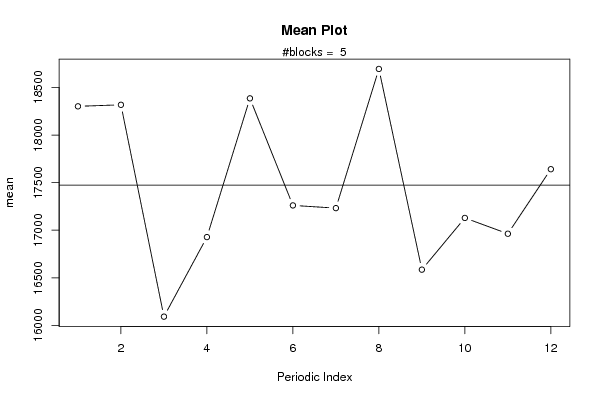
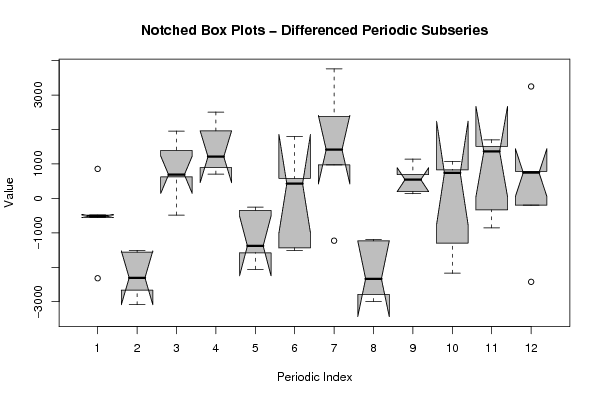
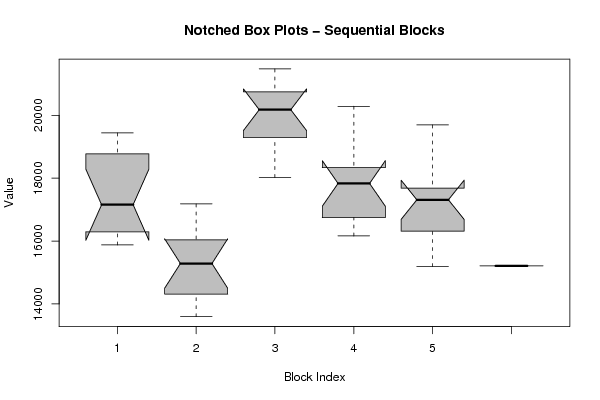
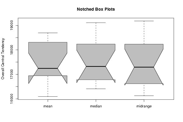
| Title produced by software | Mean Plot | ||||||||||||||||||||
| Date of computation | Fri, 24 Dec 2010 11:22:45 +0000 | ||||||||||||||||||||
| Cite this page as follows | Statistical Computations at FreeStatistics.org, Office for Research Development and Education, URL https://freestatistics.org/blog/index.php?v=date/2010/Dec/24/t1293189646cfz6imwfyu7qjnx.htm/, Retrieved Tue, 30 Apr 2024 03:11:33 +0000 | ||||||||||||||||||||
| Statistical Computations at FreeStatistics.org, Office for Research Development and Education, URL https://freestatistics.org/blog/index.php?pk=114770, Retrieved Tue, 30 Apr 2024 03:11:33 +0000 | |||||||||||||||||||||
| QR Codes: | |||||||||||||||||||||
|
| |||||||||||||||||||||
| Original text written by user: | |||||||||||||||||||||
| IsPrivate? | No (this computation is public) | ||||||||||||||||||||
| User-defined keywords | |||||||||||||||||||||
| Estimated Impact | 136 | ||||||||||||||||||||
Tree of Dependent Computations | |||||||||||||||||||||
| Family? (F = Feedback message, R = changed R code, M = changed R Module, P = changed Parameters, D = changed Data) | |||||||||||||||||||||
| - [Mean Plot] [] [2009-12-13 11:06:09] [ebd107afac1bd6180acb277edd05815b] - D [Mean Plot] [] [2010-12-24 11:22:45] [817f44ab92560f82acbc5e6c80d9a294] [Current] | |||||||||||||||||||||
| Feedback Forum | |||||||||||||||||||||
Post a new message | |||||||||||||||||||||
Dataset | |||||||||||||||||||||
| Dataseries X: | |||||||||||||||||||||
19437,5 18885,1 16579,0 17203,6 19165,7 17107,6 17690,5 18664,9 15878,6 16014,6 16842,6 15986,9 16773,3 16263,1 13597,3 14285,6 15496,8 13916,8 14345,5 15761,3 14531,6 15076,6 15816,8 17180,4 20432,3 21289,5 18203,6 20159,5 21053,2 19673,6 21473,3 20244,7 19049,6 20194,3 18021,9 19537,3 20286,6 17967,7 16409,9 17802,7 18509,9 18161,3 16721,3 19106,9 16772,1 17463,6 16162,3 17862,9 17664,9 17180,8 15672,7 15189,8 17699,4 17444,6 15930,7 19691,6 16698,0 16896,2 17972,4 17637,4 15214,0 | |||||||||||||||||||||
Tables (Output of Computation) | |||||||||||||||||||||
| |||||||||||||||||||||
Figures (Output of Computation) | |||||||||||||||||||||
Input Parameters & R Code | |||||||||||||||||||||
| Parameters (Session): | |||||||||||||||||||||
| par1 = 12 ; | |||||||||||||||||||||
| Parameters (R input): | |||||||||||||||||||||
| par1 = 12 ; | |||||||||||||||||||||
| R code (references can be found in the software module): | |||||||||||||||||||||
par1 <- as.numeric(par1) | |||||||||||||||||||||