Free Statistics
of Irreproducible Research!
Description of Statistical Computation | |||||||||||||||||||||||||||||||||||||||||||||||||||||||||||||||||||||||||||||||||||||||||||||||||||||||||||||||||||||||||||||||||
|---|---|---|---|---|---|---|---|---|---|---|---|---|---|---|---|---|---|---|---|---|---|---|---|---|---|---|---|---|---|---|---|---|---|---|---|---|---|---|---|---|---|---|---|---|---|---|---|---|---|---|---|---|---|---|---|---|---|---|---|---|---|---|---|---|---|---|---|---|---|---|---|---|---|---|---|---|---|---|---|---|---|---|---|---|---|---|---|---|---|---|---|---|---|---|---|---|---|---|---|---|---|---|---|---|---|---|---|---|---|---|---|---|---|---|---|---|---|---|---|---|---|---|---|---|---|---|---|---|---|
| Author's title | |||||||||||||||||||||||||||||||||||||||||||||||||||||||||||||||||||||||||||||||||||||||||||||||||||||||||||||||||||||||||||||||||
| Author | *The author of this computation has been verified* | ||||||||||||||||||||||||||||||||||||||||||||||||||||||||||||||||||||||||||||||||||||||||||||||||||||||||||||||||||||||||||||||||
| R Software Module | rwasp_regression_trees1.wasp | ||||||||||||||||||||||||||||||||||||||||||||||||||||||||||||||||||||||||||||||||||||||||||||||||||||||||||||||||||||||||||||||||
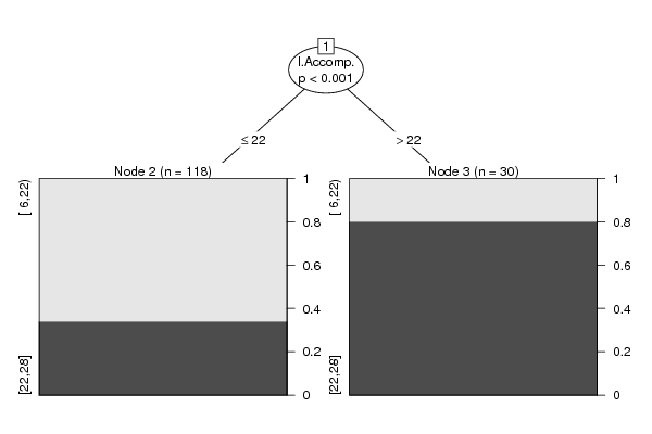
| Title produced by software | Recursive Partitioning (Regression Trees) | ||||||||||||||||||||||||||||||||||||||||||||||||||||||||||||||||||||||||||||||||||||||||||||||||||||||||||||||||||||||||||||||||
| Date of computation | Fri, 24 Dec 2010 10:41:56 +0000 | ||||||||||||||||||||||||||||||||||||||||||||||||||||||||||||||||||||||||||||||||||||||||||||||||||||||||||||||||||||||||||||||||
| Cite this page as follows | Statistical Computations at FreeStatistics.org, Office for Research Development and Education, URL https://freestatistics.org/blog/index.php?v=date/2010/Dec/24/t1293187227uwx7ysufumihw8j.htm/, Retrieved Tue, 30 Apr 2024 07:15:25 +0000 | ||||||||||||||||||||||||||||||||||||||||||||||||||||||||||||||||||||||||||||||||||||||||||||||||||||||||||||||||||||||||||||||||
| Statistical Computations at FreeStatistics.org, Office for Research Development and Education, URL https://freestatistics.org/blog/index.php?pk=114727, Retrieved Tue, 30 Apr 2024 07:15:25 +0000 | |||||||||||||||||||||||||||||||||||||||||||||||||||||||||||||||||||||||||||||||||||||||||||||||||||||||||||||||||||||||||||||||||
| QR Codes: | |||||||||||||||||||||||||||||||||||||||||||||||||||||||||||||||||||||||||||||||||||||||||||||||||||||||||||||||||||||||||||||||||
|
| |||||||||||||||||||||||||||||||||||||||||||||||||||||||||||||||||||||||||||||||||||||||||||||||||||||||||||||||||||||||||||||||||
| Original text written by user: | |||||||||||||||||||||||||||||||||||||||||||||||||||||||||||||||||||||||||||||||||||||||||||||||||||||||||||||||||||||||||||||||||
| IsPrivate? | No (this computation is public) | ||||||||||||||||||||||||||||||||||||||||||||||||||||||||||||||||||||||||||||||||||||||||||||||||||||||||||||||||||||||||||||||||
| User-defined keywords | |||||||||||||||||||||||||||||||||||||||||||||||||||||||||||||||||||||||||||||||||||||||||||||||||||||||||||||||||||||||||||||||||
| Estimated Impact | 107 | ||||||||||||||||||||||||||||||||||||||||||||||||||||||||||||||||||||||||||||||||||||||||||||||||||||||||||||||||||||||||||||||||
Tree of Dependent Computations | |||||||||||||||||||||||||||||||||||||||||||||||||||||||||||||||||||||||||||||||||||||||||||||||||||||||||||||||||||||||||||||||||
| Family? (F = Feedback message, R = changed R code, M = changed R Module, P = changed Parameters, D = changed Data) | |||||||||||||||||||||||||||||||||||||||||||||||||||||||||||||||||||||||||||||||||||||||||||||||||||||||||||||||||||||||||||||||||
| - [Recursive Partitioning (Regression Trees)] [] [2010-12-05 18:59:57] [b98453cac15ba1066b407e146608df68] - PD [Recursive Partitioning (Regression Trees)] [] [2010-12-10 15:32:27] [39e83c7b0ac936e906a817a1bb402750] - P [Recursive Partitioning (Regression Trees)] [] [2010-12-10 16:48:18] [39e83c7b0ac936e906a817a1bb402750] - P [Recursive Partitioning (Regression Trees)] [] [2010-12-10 17:49:01] [39e83c7b0ac936e906a817a1bb402750] - PD [Recursive Partitioning (Regression Trees)] [] [2010-12-21 12:59:30] [39e83c7b0ac936e906a817a1bb402750] - D [Recursive Partitioning (Regression Trees)] [] [2010-12-24 10:41:56] [558c060a42ec367ec2c020fab85c25c7] [Current] | |||||||||||||||||||||||||||||||||||||||||||||||||||||||||||||||||||||||||||||||||||||||||||||||||||||||||||||||||||||||||||||||||
| Feedback Forum | |||||||||||||||||||||||||||||||||||||||||||||||||||||||||||||||||||||||||||||||||||||||||||||||||||||||||||||||||||||||||||||||||
Post a new message | |||||||||||||||||||||||||||||||||||||||||||||||||||||||||||||||||||||||||||||||||||||||||||||||||||||||||||||||||||||||||||||||||
Dataset | |||||||||||||||||||||||||||||||||||||||||||||||||||||||||||||||||||||||||||||||||||||||||||||||||||||||||||||||||||||||||||||||||
| Dataseries X: | |||||||||||||||||||||||||||||||||||||||||||||||||||||||||||||||||||||||||||||||||||||||||||||||||||||||||||||||||||||||||||||||||
13 11 23 1 6 12 22 24 2 5 26 23 24 2 20 16 21 21 2 12 18 19 21 2 11 12 12 19 2 12 18 24 12 1 11 20 21 21 1 9 18 21 25 2 13 24 26 27 2 9 17 18 21 1 14 19 21 27 1 12 12 22 20 1 18 25 26 16 2 9 23 20 26 1 15 22 20 24 2 12 23 26 25 2 12 16 27 25 1 12 16 27 27 1 15 15 16 23 2 11 24 26 22 1 13 18 20 10 1 10 23 25 25 2 17 18 16 18 1 13 19 20 21 1 17 17 20 20 1 15 22 24 18 1 13 22 24 25 1 17 8 22 28 1 21 12 18 27 1 12 22 21 20 2 12 16 17 20 1 15 12 15 20 2 8 28 28 27 2 15 15 23 23 1 16 17 19 23 2 9 16 15 22 2 13 24 26 26 1 11 27 20 21 1 9 10 11 17 1 15 20 17 27 2 9 17 16 16 2 15 20 21 26 1 14 16 18 17 1 8 16 17 24 2 11 22 21 23 2 14 19 18 20 1 14 11 16 10 1 12 11 13 21 1 15 28 28 25 1 11 12 25 28 1 11 22 24 25 2 9 15 15 20 2 8 19 21 20 1 13 12 11 27 1 12 18 27 26 1 24 21 23 19 2 11 21 21 26 1 11 15 16 20 2 16 12 20 22 1 12 25 21 19 2 18 12 10 23 2 12 25 18 28 2 14 17 20 22 2 16 26 21 27 2 24 24 24 14 1 13 18 26 25 1 11 20 23 22 1 14 17 22 24 1 16 11 13 23 1 12 27 27 25 1 21 14 24 28 2 11 22 19 28 1 6 19 17 16 2 9 19 16 25 1 14 18 20 21 1 16 9 8 27 1 18 22 16 21 2 9 17 17 22 1 13 23 23 26 2 17 16 18 21 1 11 23 24 24 1 16 13 17 24 1 11 21 20 23 1 11 17 22 26 2 11 15 22 21 1 20 16 20 24 1 10 19 18 23 1 12 19 21 21 2 11 16 23 20 1 14 23 28 22 1 12 19 19 26 1 12 17 22 23 1 12 20 17 23 2 10 25 25 22 2 12 22 22 25 2 10 18 21 21 2 10 16 15 21 1 13 18 20 25 1 12 15 25 26 2 13 19 21 21 1 9 23 24 24 1 14 20 23 21 2 14 24 22 23 1 12 17 14 24 1 18 20 11 24 1 17 11 22 24 1 12 20 22 25 1 15 8 6 28 1 8 22 15 18 2 8 20 26 28 1 12 23 26 22 1 10 11 20 28 1 18 22 26 22 1 15 10 15 24 1 16 19 25 27 2 11 26 22 21 2 10 22 20 26 2 7 12 18 24 1 17 13 23 25 1 7 19 22 20 2 14 19 23 21 1 12 21 17 23 1 15 11 20 23 1 13 21 21 19 2 10 25 23 22 1 16 27 25 15 2 11 21 25 24 2 7 14 21 18 2 15 16 22 18 1 18 16 18 23 1 11 19 18 17 1 13 24 18 19 2 11 18 21 21 2 13 16 21 12 2 12 20 25 25 2 11 19 24 25 1 11 20 24 24 1 13 27 28 24 2 8 24 24 24 2 12 23 22 22 2 9 20 22 22 1 14 20 20 21 1 18 20 25 23 1 15 15 13 21 1 9 17 21 24 1 11 16 23 22 1 17 20 18 25 2 12 | |||||||||||||||||||||||||||||||||||||||||||||||||||||||||||||||||||||||||||||||||||||||||||||||||||||||||||||||||||||||||||||||||
Tables (Output of Computation) | |||||||||||||||||||||||||||||||||||||||||||||||||||||||||||||||||||||||||||||||||||||||||||||||||||||||||||||||||||||||||||||||||
| |||||||||||||||||||||||||||||||||||||||||||||||||||||||||||||||||||||||||||||||||||||||||||||||||||||||||||||||||||||||||||||||||
Figures (Output of Computation) | |||||||||||||||||||||||||||||||||||||||||||||||||||||||||||||||||||||||||||||||||||||||||||||||||||||||||||||||||||||||||||||||||
Input Parameters & R Code | |||||||||||||||||||||||||||||||||||||||||||||||||||||||||||||||||||||||||||||||||||||||||||||||||||||||||||||||||||||||||||||||||
| Parameters (Session): | |||||||||||||||||||||||||||||||||||||||||||||||||||||||||||||||||||||||||||||||||||||||||||||||||||||||||||||||||||||||||||||||||
| par1 = 2 ; par2 = quantiles ; par3 = 2 ; par4 = yes ; | |||||||||||||||||||||||||||||||||||||||||||||||||||||||||||||||||||||||||||||||||||||||||||||||||||||||||||||||||||||||||||||||||
| Parameters (R input): | |||||||||||||||||||||||||||||||||||||||||||||||||||||||||||||||||||||||||||||||||||||||||||||||||||||||||||||||||||||||||||||||||
| par1 = 2 ; par2 = quantiles ; par3 = 2 ; par4 = yes ; | |||||||||||||||||||||||||||||||||||||||||||||||||||||||||||||||||||||||||||||||||||||||||||||||||||||||||||||||||||||||||||||||||
| R code (references can be found in the software module): | |||||||||||||||||||||||||||||||||||||||||||||||||||||||||||||||||||||||||||||||||||||||||||||||||||||||||||||||||||||||||||||||||
library(party) | |||||||||||||||||||||||||||||||||||||||||||||||||||||||||||||||||||||||||||||||||||||||||||||||||||||||||||||||||||||||||||||||||