Free Statistics
of Irreproducible Research!
Description of Statistical Computation | |||||||||||||||||||||
|---|---|---|---|---|---|---|---|---|---|---|---|---|---|---|---|---|---|---|---|---|---|
| Author's title | |||||||||||||||||||||
| Author | *The author of this computation has been verified* | ||||||||||||||||||||
| R Software Module | rwasp_meanplot.wasp | ||||||||||||||||||||
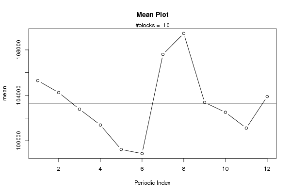
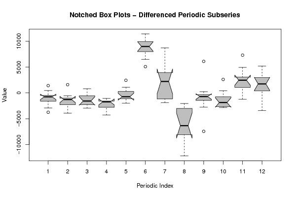
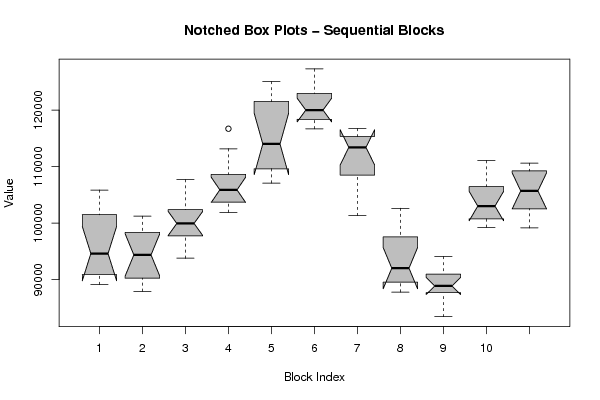
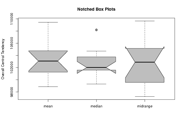
| Title produced by software | Mean Plot | ||||||||||||||||||||
| Date of computation | Fri, 24 Dec 2010 10:35:44 +0000 | ||||||||||||||||||||
| Cite this page as follows | Statistical Computations at FreeStatistics.org, Office for Research Development and Education, URL https://freestatistics.org/blog/index.php?v=date/2010/Dec/24/t1293186821ipz83e1lu91sevr.htm/, Retrieved Tue, 30 Apr 2024 04:49:52 +0000 | ||||||||||||||||||||
| Statistical Computations at FreeStatistics.org, Office for Research Development and Education, URL https://freestatistics.org/blog/index.php?pk=114719, Retrieved Tue, 30 Apr 2024 04:49:52 +0000 | |||||||||||||||||||||
| QR Codes: | |||||||||||||||||||||
|
| |||||||||||||||||||||
| Original text written by user: | |||||||||||||||||||||
| IsPrivate? | No (this computation is public) | ||||||||||||||||||||
| User-defined keywords | |||||||||||||||||||||
| Estimated Impact | 140 | ||||||||||||||||||||
Tree of Dependent Computations | |||||||||||||||||||||
| Family? (F = Feedback message, R = changed R code, M = changed R Module, P = changed Parameters, D = changed Data) | |||||||||||||||||||||
| - [Mean Plot] [middengeschoolden] [2010-12-24 10:13:59] [8214fe6d084e5ad7598b249a26cc9f06] - D [Mean Plot] [laaggschoolden] [2010-12-24 10:35:44] [b47314d83d48c7bf812ec2bcd743b159] [Current] | |||||||||||||||||||||
| Feedback Forum | |||||||||||||||||||||
Post a new message | |||||||||||||||||||||
Dataset | |||||||||||||||||||||
| Dataseries X: | |||||||||||||||||||||
104708 101817 97898 95559 92822 90848 101141 105841 93647 90923 89130 90212 93196 91861 90593 89895 88819 87924 96906 101217 98709 98139 95529 98577 100772 100180 99200 96251 94514 93780 105192 107682 99687 99436 102049 102673 105813 105056 103916 103513 101893 102503 113149 116696 108500 107800 105941 108742 111680 111270 110698 108517 107127 107088 116321 125045 116779 122887 120162 123198 123610 122293 121289 119393 117494 116693 125062 127281 120195 119804 117113 119240 115823 116281 113816 114632 112987 111633 116721 114850 112797 105368 102524 101327 102612 98873 95993 93244 90403 88539 98106 96963 90781 89253 87794 89810 90864 89025 87621 87718 83433 84535 92223 91052 88456 88706 89137 94066 99258 100673 102269 100833 99314 101764 108242 108148 104761 103772 103737 111043 109906 109335 107247 105690 102755 102280 110590 109122 102803 101424 99138 | |||||||||||||||||||||
Tables (Output of Computation) | |||||||||||||||||||||
| |||||||||||||||||||||
Figures (Output of Computation) | |||||||||||||||||||||
Input Parameters & R Code | |||||||||||||||||||||
| Parameters (Session): | |||||||||||||||||||||
| par1 = 12 ; | |||||||||||||||||||||
| Parameters (R input): | |||||||||||||||||||||
| par1 = 12 ; | |||||||||||||||||||||
| R code (references can be found in the software module): | |||||||||||||||||||||
par1 <- as.numeric(par1) | |||||||||||||||||||||