Repository of Reproducible Computations

Free Statistics

of Irreproducible Research!

Author's title

Author

*The author of this computation has been verified*

R Software Module

rwasp_autocorrelation.wasp

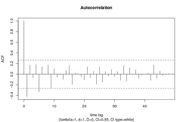
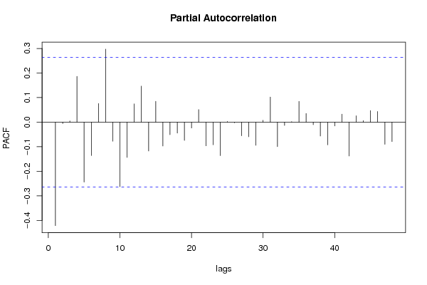
Title produced by software

(Partial) Autocorrelation Function

Date of computation

Fri, 24 Dec 2010 10:04:57 +0000

Cite this page as follows

Statistical Computations at FreeStatistics.org, Office for Research Development and Education, URL https://freestatistics.org/blog/index.php?v=date/2010/Dec/24/t12931850433xplnj54saw35ma.htm/, Retrieved Tue, 30 Apr 2024 00:58:53 +0000

Statistical Computations at FreeStatistics.org, Office for Research Development and Education, URL https://freestatistics.org/blog/index.php?pk=114686, Retrieved Tue, 30 Apr 2024 00:58:53 +0000

QR Codes:

Paste this QR Code to cite your computation.

Original text written by user:

IsPrivate?

No (this computation is public)

User-defined keywords

Estimated Impact

158

Family? (F = Feedback message, R = changed R code, M = changed R Module, P = changed Parameters, D = changed Data)

-     [Univariate Explorative Data Analysis] [Run Sequence gebo...] [2008-12-12 13:32:37] [76963dc1903f0f612b6153510a3818cf]
- R  D  [Univariate Explorative Data Analysis] [Run Sequence gebo...] [2008-12-17 12:14:40] [76963dc1903f0f612b6153510a3818cf]
-         [Univariate Explorative Data Analysis] [Run Sequence Plot...] [2008-12-22 18:19:51] [1ce0d16c8f4225c977b42c8fa93bc163]
- RMP       [(Partial) Autocorrelation Function] [Identifying Integ...] [2009-11-22 12:16:10] [b98453cac15ba1066b407e146608df68]
-    D        [(Partial) Autocorrelation Function] [Model 1 (d = 0, D...] [2009-11-24 17:27:24] [ee7c2e7343f5b1451e62c5c16ec521f1]
-    D          [(Partial) Autocorrelation Function] [Methode 1 (D=0, d=0)] [2009-11-27 12:01:23] [76ab39dc7a55316678260825bd5ad46c]
-    D            [(Partial) Autocorrelation Function] [methode 1 (d=0 D= 0)] [2009-11-27 20:21:42] [4b453aa14d54730625f8d3de5f1f6d82]
-    D              [(Partial) Autocorrelation Function] [koffie en thee] [2009-12-16 19:04:55] [7773f496f69461f4a67891f0ef752622]
-    D                [(Partial) Autocorrelation Function] [Appelen Jonagold ...] [2009-12-17 16:51:16] [7773f496f69461f4a67891f0ef752622]
-   PD                  [(Partial) Autocorrelation Function] [ACFKoffie] [2010-12-20 13:05:39] [3fb95cad3bbcce10c72dbbcc5bec5662]
-   PD                      [(Partial) Autocorrelation Function] [ACFKoffied1] [2010-12-24 10:04:57] [9be3691a9b6ce074cb51fd18377fce28] [Current]

Feedback Forum

Post a new message

Dataseries X:

Download CSV

Histogram

Boxplots

1.64
1.65
1.65
1.65
1.66
1.66
1.67
1.67
1.68
1.68
1.68
1.68
1.69
1.69
1.7
1.7
1.71
1.71
1.71
1.71
1.72
1.72
1.72
1.73
1.73
1.73
1.74
1.75
1.75
1.76
1.76
1.77
1.77
1.78
1.79
1.8
1.8
1.81
1.81
1.81
1.81
1.82
1.82
1.82
1.83
1.83
1.83
1.84
1.84
1.85
1.85
1.86
1.86
1.86
1.86
1.86

Summary of computational transaction
Raw Input	view raw input (R code)
Raw Output	view raw output of R engine
Computing time	21 seconds
R Server	'George Udny Yule' @ 72.249.76.132

\begin{tabular}{lllllllll}
\hline
Summary of computational transaction \tabularnewline
Raw Input & view raw input (R code)  \tabularnewline
Raw Output & view raw output of R engine  \tabularnewline
Computing time & 21 seconds \tabularnewline
R Server & 'George Udny Yule' @ 72.249.76.132 \tabularnewline
\hline
\end{tabular}
%Source: https://freestatistics.org/blog/index.php?pk=114686&T=0

[TABLE]
[ROW][C]Summary of computational transaction[/C][/ROW]
[ROW][C]Raw Input[/C][C]view raw input (R code) [/C][/ROW]
[ROW][C]Raw Output[/C][C]view raw output of R engine [/C][/ROW]
[ROW][C]Computing time[/C][C]21 seconds[/C][/ROW]
[ROW][C]R Server[/C][C]'George Udny Yule' @ 72.249.76.132[/C][/ROW]
[/TABLE]
Source: https://freestatistics.org/blog/index.php?pk=114686&T=0

Globally Unique Identifier (entire table): ba.freestatistics.org/blog/index.php?pk=114686&T=0

As an alternative you can also use a QR Code:

The GUIDs for individual cells are displayed in the table below:

Summary of computational transaction
Raw Input	view raw input (R code)
Raw Output	view raw output of R engine
Computing time	21 seconds
R Server	'George Udny Yule' @ 72.249.76.132

Autocorrelation Function
Time lag k	ACF(k)	T-STAT	P-value
1	-0.421212	-3.1238	0.001424
2	0.172727	1.281	0.102788
3	-0.066667	-0.4944	0.311492
4	0.178788	1.3259	0.095172
5	-0.333333	-2.4721	0.008278
6	0.139394	1.0338	0.152883
7	0.006061	0.0449	0.482156
8	0.175758	1.3035	0.098925
9	-0.260606	-1.9327	0.029214
10	0.106061	0.7866	0.217456
11	-0.057576	-0.427	0.335526
12	-0.009091	-0.0674	0.473246
13	-0.09697	-0.7191	0.237548
14	0.072727	0.5394	0.295908
15	0.166667	1.236	0.11085
16	-0.193939	-1.4383	0.078009
17	0.021212	0.1573	0.437787
18	0.009091	0.0674	0.473246
19	-0.048485	-0.3596	0.360272
20	-0.106061	-0.7866	0.217456
21	0.139394	1.0338	0.152883
22	-0.069697	-0.5169	0.303654
23	0.054545	0.4045	0.3437
24	-0.184848	-1.3709	0.087992
25	0.136364	1.0113	0.158151
26	-0.148485	-1.1012	0.137804
27	0.051515	0.382	0.35195
28	-0.036364	-0.2697	0.394208
29	0.087879	0.6517	0.258646
30	-0.045455	-0.3371	0.368662
31	0.048485	0.3596	0.360272
32	-0.115152	-0.854	0.198408
33	0.160606	1.1911	0.119367
34	-0.124242	-0.9214	0.180431
35	0.121212	0.8989	0.186304
36	-0.012121	-0.0899	0.464349
37	0.081818	0.6068	0.273247
38	-0.081818	-0.6068	0.273247
39	-0.018182	-0.1348	0.446615
40	0	0	0.5
41	0.018182	0.1348	0.446615
42	-0.115152	-0.854	0.198408
43	0.175758	1.3035	0.098925
44	-0.078788	-0.5843	0.280702
45	0.060606	0.4495	0.327431
46	-0.027273	-0.2023	0.42023
47	-0.009091	-0.0674	0.473246
48	0.009091	0.0674	0.473246

\begin{tabular}{lllllllll}
\hline
Autocorrelation Function \tabularnewline
Time lag k & ACF(k) & T-STAT & P-value \tabularnewline
1 & -0.421212 & -3.1238 & 0.001424 \tabularnewline
2 & 0.172727 & 1.281 & 0.102788 \tabularnewline
3 & -0.066667 & -0.4944 & 0.311492 \tabularnewline
4 & 0.178788 & 1.3259 & 0.095172 \tabularnewline
5 & -0.333333 & -2.4721 & 0.008278 \tabularnewline
6 & 0.139394 & 1.0338 & 0.152883 \tabularnewline
7 & 0.006061 & 0.0449 & 0.482156 \tabularnewline
8 & 0.175758 & 1.3035 & 0.098925 \tabularnewline
9 & -0.260606 & -1.9327 & 0.029214 \tabularnewline
10 & 0.106061 & 0.7866 & 0.217456 \tabularnewline
11 & -0.057576 & -0.427 & 0.335526 \tabularnewline
12 & -0.009091 & -0.0674 & 0.473246 \tabularnewline
13 & -0.09697 & -0.7191 & 0.237548 \tabularnewline
14 & 0.072727 & 0.5394 & 0.295908 \tabularnewline
15 & 0.166667 & 1.236 & 0.11085 \tabularnewline
16 & -0.193939 & -1.4383 & 0.078009 \tabularnewline
17 & 0.021212 & 0.1573 & 0.437787 \tabularnewline
18 & 0.009091 & 0.0674 & 0.473246 \tabularnewline
19 & -0.048485 & -0.3596 & 0.360272 \tabularnewline
20 & -0.106061 & -0.7866 & 0.217456 \tabularnewline
21 & 0.139394 & 1.0338 & 0.152883 \tabularnewline
22 & -0.069697 & -0.5169 & 0.303654 \tabularnewline
23 & 0.054545 & 0.4045 & 0.3437 \tabularnewline
24 & -0.184848 & -1.3709 & 0.087992 \tabularnewline
25 & 0.136364 & 1.0113 & 0.158151 \tabularnewline
26 & -0.148485 & -1.1012 & 0.137804 \tabularnewline
27 & 0.051515 & 0.382 & 0.35195 \tabularnewline
28 & -0.036364 & -0.2697 & 0.394208 \tabularnewline
29 & 0.087879 & 0.6517 & 0.258646 \tabularnewline
30 & -0.045455 & -0.3371 & 0.368662 \tabularnewline
31 & 0.048485 & 0.3596 & 0.360272 \tabularnewline
32 & -0.115152 & -0.854 & 0.198408 \tabularnewline
33 & 0.160606 & 1.1911 & 0.119367 \tabularnewline
34 & -0.124242 & -0.9214 & 0.180431 \tabularnewline
35 & 0.121212 & 0.8989 & 0.186304 \tabularnewline
36 & -0.012121 & -0.0899 & 0.464349 \tabularnewline
37 & 0.081818 & 0.6068 & 0.273247 \tabularnewline
38 & -0.081818 & -0.6068 & 0.273247 \tabularnewline
39 & -0.018182 & -0.1348 & 0.446615 \tabularnewline
40 & 0 & 0 & 0.5 \tabularnewline
41 & 0.018182 & 0.1348 & 0.446615 \tabularnewline
42 & -0.115152 & -0.854 & 0.198408 \tabularnewline
43 & 0.175758 & 1.3035 & 0.098925 \tabularnewline
44 & -0.078788 & -0.5843 & 0.280702 \tabularnewline
45 & 0.060606 & 0.4495 & 0.327431 \tabularnewline
46 & -0.027273 & -0.2023 & 0.42023 \tabularnewline
47 & -0.009091 & -0.0674 & 0.473246 \tabularnewline
48 & 0.009091 & 0.0674 & 0.473246 \tabularnewline
\hline
\end{tabular}
%Source: https://freestatistics.org/blog/index.php?pk=114686&T=1

[TABLE]
[ROW][C]Autocorrelation Function[/C][/ROW]
[ROW][C]Time lag k[/C][C]ACF(k)[/C][C]T-STAT[/C][C]P-value[/C][/ROW]
[ROW][C]1[/C][C]-0.421212[/C][C]-3.1238[/C][C]0.001424[/C][/ROW]
[ROW][C]2[/C][C]0.172727[/C][C]1.281[/C][C]0.102788[/C][/ROW]
[ROW][C]3[/C][C]-0.066667[/C][C]-0.4944[/C][C]0.311492[/C][/ROW]
[ROW][C]4[/C][C]0.178788[/C][C]1.3259[/C][C]0.095172[/C][/ROW]
[ROW][C]5[/C][C]-0.333333[/C][C]-2.4721[/C][C]0.008278[/C][/ROW]
[ROW][C]6[/C][C]0.139394[/C][C]1.0338[/C][C]0.152883[/C][/ROW]
[ROW][C]7[/C][C]0.006061[/C][C]0.0449[/C][C]0.482156[/C][/ROW]
[ROW][C]8[/C][C]0.175758[/C][C]1.3035[/C][C]0.098925[/C][/ROW]
[ROW][C]9[/C][C]-0.260606[/C][C]-1.9327[/C][C]0.029214[/C][/ROW]
[ROW][C]10[/C][C]0.106061[/C][C]0.7866[/C][C]0.217456[/C][/ROW]
[ROW][C]11[/C][C]-0.057576[/C][C]-0.427[/C][C]0.335526[/C][/ROW]
[ROW][C]12[/C][C]-0.009091[/C][C]-0.0674[/C][C]0.473246[/C][/ROW]
[ROW][C]13[/C][C]-0.09697[/C][C]-0.7191[/C][C]0.237548[/C][/ROW]
[ROW][C]14[/C][C]0.072727[/C][C]0.5394[/C][C]0.295908[/C][/ROW]
[ROW][C]15[/C][C]0.166667[/C][C]1.236[/C][C]0.11085[/C][/ROW]
[ROW][C]16[/C][C]-0.193939[/C][C]-1.4383[/C][C]0.078009[/C][/ROW]
[ROW][C]17[/C][C]0.021212[/C][C]0.1573[/C][C]0.437787[/C][/ROW]
[ROW][C]18[/C][C]0.009091[/C][C]0.0674[/C][C]0.473246[/C][/ROW]
[ROW][C]19[/C][C]-0.048485[/C][C]-0.3596[/C][C]0.360272[/C][/ROW]
[ROW][C]20[/C][C]-0.106061[/C][C]-0.7866[/C][C]0.217456[/C][/ROW]
[ROW][C]21[/C][C]0.139394[/C][C]1.0338[/C][C]0.152883[/C][/ROW]
[ROW][C]22[/C][C]-0.069697[/C][C]-0.5169[/C][C]0.303654[/C][/ROW]
[ROW][C]23[/C][C]0.054545[/C][C]0.4045[/C][C]0.3437[/C][/ROW]
[ROW][C]24[/C][C]-0.184848[/C][C]-1.3709[/C][C]0.087992[/C][/ROW]
[ROW][C]25[/C][C]0.136364[/C][C]1.0113[/C][C]0.158151[/C][/ROW]
[ROW][C]26[/C][C]-0.148485[/C][C]-1.1012[/C][C]0.137804[/C][/ROW]
[ROW][C]27[/C][C]0.051515[/C][C]0.382[/C][C]0.35195[/C][/ROW]
[ROW][C]28[/C][C]-0.036364[/C][C]-0.2697[/C][C]0.394208[/C][/ROW]
[ROW][C]29[/C][C]0.087879[/C][C]0.6517[/C][C]0.258646[/C][/ROW]
[ROW][C]30[/C][C]-0.045455[/C][C]-0.3371[/C][C]0.368662[/C][/ROW]
[ROW][C]31[/C][C]0.048485[/C][C]0.3596[/C][C]0.360272[/C][/ROW]
[ROW][C]32[/C][C]-0.115152[/C][C]-0.854[/C][C]0.198408[/C][/ROW]
[ROW][C]33[/C][C]0.160606[/C][C]1.1911[/C][C]0.119367[/C][/ROW]
[ROW][C]34[/C][C]-0.124242[/C][C]-0.9214[/C][C]0.180431[/C][/ROW]
[ROW][C]35[/C][C]0.121212[/C][C]0.8989[/C][C]0.186304[/C][/ROW]
[ROW][C]36[/C][C]-0.012121[/C][C]-0.0899[/C][C]0.464349[/C][/ROW]
[ROW][C]37[/C][C]0.081818[/C][C]0.6068[/C][C]0.273247[/C][/ROW]
[ROW][C]38[/C][C]-0.081818[/C][C]-0.6068[/C][C]0.273247[/C][/ROW]
[ROW][C]39[/C][C]-0.018182[/C][C]-0.1348[/C][C]0.446615[/C][/ROW]
[ROW][C]40[/C][C]0[/C][C]0[/C][C]0.5[/C][/ROW]
[ROW][C]41[/C][C]0.018182[/C][C]0.1348[/C][C]0.446615[/C][/ROW]
[ROW][C]42[/C][C]-0.115152[/C][C]-0.854[/C][C]0.198408[/C][/ROW]
[ROW][C]43[/C][C]0.175758[/C][C]1.3035[/C][C]0.098925[/C][/ROW]
[ROW][C]44[/C][C]-0.078788[/C][C]-0.5843[/C][C]0.280702[/C][/ROW]
[ROW][C]45[/C][C]0.060606[/C][C]0.4495[/C][C]0.327431[/C][/ROW]
[ROW][C]46[/C][C]-0.027273[/C][C]-0.2023[/C][C]0.42023[/C][/ROW]
[ROW][C]47[/C][C]-0.009091[/C][C]-0.0674[/C][C]0.473246[/C][/ROW]
[ROW][C]48[/C][C]0.009091[/C][C]0.0674[/C][C]0.473246[/C][/ROW]
[/TABLE]
Source: https://freestatistics.org/blog/index.php?pk=114686&T=1

Globally Unique Identifier (entire table): ba.freestatistics.org/blog/index.php?pk=114686&T=1

As an alternative you can also use a QR Code:

The GUIDs for individual cells are displayed in the table below:

Autocorrelation Function
Time lag k	ACF(k)	T-STAT	P-value
1	-0.421212	-3.1238	0.001424
2	0.172727	1.281	0.102788
3	-0.066667	-0.4944	0.311492
4	0.178788	1.3259	0.095172
5	-0.333333	-2.4721	0.008278
6	0.139394	1.0338	0.152883
7	0.006061	0.0449	0.482156
8	0.175758	1.3035	0.098925
9	-0.260606	-1.9327	0.029214
10	0.106061	0.7866	0.217456
11	-0.057576	-0.427	0.335526
12	-0.009091	-0.0674	0.473246
13	-0.09697	-0.7191	0.237548
14	0.072727	0.5394	0.295908
15	0.166667	1.236	0.11085
16	-0.193939	-1.4383	0.078009
17	0.021212	0.1573	0.437787
18	0.009091	0.0674	0.473246
19	-0.048485	-0.3596	0.360272
20	-0.106061	-0.7866	0.217456
21	0.139394	1.0338	0.152883
22	-0.069697	-0.5169	0.303654
23	0.054545	0.4045	0.3437
24	-0.184848	-1.3709	0.087992
25	0.136364	1.0113	0.158151
26	-0.148485	-1.1012	0.137804
27	0.051515	0.382	0.35195
28	-0.036364	-0.2697	0.394208
29	0.087879	0.6517	0.258646
30	-0.045455	-0.3371	0.368662
31	0.048485	0.3596	0.360272
32	-0.115152	-0.854	0.198408
33	0.160606	1.1911	0.119367
34	-0.124242	-0.9214	0.180431
35	0.121212	0.8989	0.186304
36	-0.012121	-0.0899	0.464349
37	0.081818	0.6068	0.273247
38	-0.081818	-0.6068	0.273247
39	-0.018182	-0.1348	0.446615
40	0	0	0.5
41	0.018182	0.1348	0.446615
42	-0.115152	-0.854	0.198408
43	0.175758	1.3035	0.098925
44	-0.078788	-0.5843	0.280702
45	0.060606	0.4495	0.327431
46	-0.027273	-0.2023	0.42023
47	-0.009091	-0.0674	0.473246
48	0.009091	0.0674	0.473246

Partial Autocorrelation Function
Time lag k	PACF(k)	T-STAT	P-value
1	-0.421212	-3.1238	0.001424
2	-0.005704	-0.0423	0.483204
3	0.004985	0.037	0.485322
4	0.186338	1.3819	0.086292
5	-0.243883	-1.8087	0.037984
6	-0.136032	-1.0088	0.158734
7	0.075917	0.563	0.287857
8	0.297348	2.2052	0.01582
9	-0.077449	-0.5744	0.284028
10	-0.262355	-1.9457	0.028406
11	-0.143426	-1.0637	0.146062
12	0.07442	0.5519	0.291622
13	0.146733	1.0882	0.140626
14	-0.117411	-0.8707	0.193839
15	0.084811	0.629	0.265984
16	-0.097171	-0.7206	0.237092
17	-0.051149	-0.3793	0.352953
18	-0.044713	-0.3316	0.370727
19	-0.074221	-0.5504	0.292123
20	-0.023814	-0.1766	0.430231
21	0.05102	0.3784	0.353306
22	-0.096458	-0.7154	0.238708
23	-0.092217	-0.6839	0.248454
24	-0.136379	-1.0114	0.158124
25	0.00284	0.0211	0.491636
26	-0.00252	-0.0187	0.492579
27	-0.055481	-0.4115	0.341169
28	-0.05948	-0.4411	0.330429
29	-0.094365	-0.6998	0.243491
30	0.007588	0.0563	0.477663
31	0.102279	0.7585	0.225688
32	-0.099623	-0.7388	0.231577
33	-0.013495	-0.1001	0.460322
34	0.002119	0.0157	0.493758
35	0.084719	0.6283	0.266206
36	0.035218	0.2612	0.397463
37	-0.010502	-0.0779	0.469101
38	-0.056625	-0.4199	0.338081
39	-0.092523	-0.6862	0.247745
40	-0.015407	-0.1143	0.454723
41	0.032823	0.2434	0.404293
42	-0.137586	-1.0204	0.156012
43	0.026173	0.1941	0.423405
44	0.00633	0.0469	0.481364
45	0.04708	0.3492	0.364155
46	0.043534	0.3229	0.374015
47	-0.0902	-0.6689	0.253165
48	-0.079181	-0.5872	0.279728

\begin{tabular}{lllllllll}
\hline
Partial Autocorrelation Function \tabularnewline
Time lag k & PACF(k) & T-STAT & P-value \tabularnewline
1 & -0.421212 & -3.1238 & 0.001424 \tabularnewline
2 & -0.005704 & -0.0423 & 0.483204 \tabularnewline
3 & 0.004985 & 0.037 & 0.485322 \tabularnewline
4 & 0.186338 & 1.3819 & 0.086292 \tabularnewline
5 & -0.243883 & -1.8087 & 0.037984 \tabularnewline
6 & -0.136032 & -1.0088 & 0.158734 \tabularnewline
7 & 0.075917 & 0.563 & 0.287857 \tabularnewline
8 & 0.297348 & 2.2052 & 0.01582 \tabularnewline
9 & -0.077449 & -0.5744 & 0.284028 \tabularnewline
10 & -0.262355 & -1.9457 & 0.028406 \tabularnewline
11 & -0.143426 & -1.0637 & 0.146062 \tabularnewline
12 & 0.07442 & 0.5519 & 0.291622 \tabularnewline
13 & 0.146733 & 1.0882 & 0.140626 \tabularnewline
14 & -0.117411 & -0.8707 & 0.193839 \tabularnewline
15 & 0.084811 & 0.629 & 0.265984 \tabularnewline
16 & -0.097171 & -0.7206 & 0.237092 \tabularnewline
17 & -0.051149 & -0.3793 & 0.352953 \tabularnewline
18 & -0.044713 & -0.3316 & 0.370727 \tabularnewline
19 & -0.074221 & -0.5504 & 0.292123 \tabularnewline
20 & -0.023814 & -0.1766 & 0.430231 \tabularnewline
21 & 0.05102 & 0.3784 & 0.353306 \tabularnewline
22 & -0.096458 & -0.7154 & 0.238708 \tabularnewline
23 & -0.092217 & -0.6839 & 0.248454 \tabularnewline
24 & -0.136379 & -1.0114 & 0.158124 \tabularnewline
25 & 0.00284 & 0.0211 & 0.491636 \tabularnewline
26 & -0.00252 & -0.0187 & 0.492579 \tabularnewline
27 & -0.055481 & -0.4115 & 0.341169 \tabularnewline
28 & -0.05948 & -0.4411 & 0.330429 \tabularnewline
29 & -0.094365 & -0.6998 & 0.243491 \tabularnewline
30 & 0.007588 & 0.0563 & 0.477663 \tabularnewline
31 & 0.102279 & 0.7585 & 0.225688 \tabularnewline
32 & -0.099623 & -0.7388 & 0.231577 \tabularnewline
33 & -0.013495 & -0.1001 & 0.460322 \tabularnewline
34 & 0.002119 & 0.0157 & 0.493758 \tabularnewline
35 & 0.084719 & 0.6283 & 0.266206 \tabularnewline
36 & 0.035218 & 0.2612 & 0.397463 \tabularnewline
37 & -0.010502 & -0.0779 & 0.469101 \tabularnewline
38 & -0.056625 & -0.4199 & 0.338081 \tabularnewline
39 & -0.092523 & -0.6862 & 0.247745 \tabularnewline
40 & -0.015407 & -0.1143 & 0.454723 \tabularnewline
41 & 0.032823 & 0.2434 & 0.404293 \tabularnewline
42 & -0.137586 & -1.0204 & 0.156012 \tabularnewline
43 & 0.026173 & 0.1941 & 0.423405 \tabularnewline
44 & 0.00633 & 0.0469 & 0.481364 \tabularnewline
45 & 0.04708 & 0.3492 & 0.364155 \tabularnewline
46 & 0.043534 & 0.3229 & 0.374015 \tabularnewline
47 & -0.0902 & -0.6689 & 0.253165 \tabularnewline
48 & -0.079181 & -0.5872 & 0.279728 \tabularnewline
\hline
\end{tabular}
%Source: https://freestatistics.org/blog/index.php?pk=114686&T=2

[TABLE]
[ROW][C]Partial Autocorrelation Function[/C][/ROW]
[ROW][C]Time lag k[/C][C]PACF(k)[/C][C]T-STAT[/C][C]P-value[/C][/ROW]
[ROW][C]1[/C][C]-0.421212[/C][C]-3.1238[/C][C]0.001424[/C][/ROW]
[ROW][C]2[/C][C]-0.005704[/C][C]-0.0423[/C][C]0.483204[/C][/ROW]
[ROW][C]3[/C][C]0.004985[/C][C]0.037[/C][C]0.485322[/C][/ROW]
[ROW][C]4[/C][C]0.186338[/C][C]1.3819[/C][C]0.086292[/C][/ROW]
[ROW][C]5[/C][C]-0.243883[/C][C]-1.8087[/C][C]0.037984[/C][/ROW]
[ROW][C]6[/C][C]-0.136032[/C][C]-1.0088[/C][C]0.158734[/C][/ROW]
[ROW][C]7[/C][C]0.075917[/C][C]0.563[/C][C]0.287857[/C][/ROW]
[ROW][C]8[/C][C]0.297348[/C][C]2.2052[/C][C]0.01582[/C][/ROW]
[ROW][C]9[/C][C]-0.077449[/C][C]-0.5744[/C][C]0.284028[/C][/ROW]
[ROW][C]10[/C][C]-0.262355[/C][C]-1.9457[/C][C]0.028406[/C][/ROW]
[ROW][C]11[/C][C]-0.143426[/C][C]-1.0637[/C][C]0.146062[/C][/ROW]
[ROW][C]12[/C][C]0.07442[/C][C]0.5519[/C][C]0.291622[/C][/ROW]
[ROW][C]13[/C][C]0.146733[/C][C]1.0882[/C][C]0.140626[/C][/ROW]
[ROW][C]14[/C][C]-0.117411[/C][C]-0.8707[/C][C]0.193839[/C][/ROW]
[ROW][C]15[/C][C]0.084811[/C][C]0.629[/C][C]0.265984[/C][/ROW]
[ROW][C]16[/C][C]-0.097171[/C][C]-0.7206[/C][C]0.237092[/C][/ROW]
[ROW][C]17[/C][C]-0.051149[/C][C]-0.3793[/C][C]0.352953[/C][/ROW]
[ROW][C]18[/C][C]-0.044713[/C][C]-0.3316[/C][C]0.370727[/C][/ROW]
[ROW][C]19[/C][C]-0.074221[/C][C]-0.5504[/C][C]0.292123[/C][/ROW]
[ROW][C]20[/C][C]-0.023814[/C][C]-0.1766[/C][C]0.430231[/C][/ROW]
[ROW][C]21[/C][C]0.05102[/C][C]0.3784[/C][C]0.353306[/C][/ROW]
[ROW][C]22[/C][C]-0.096458[/C][C]-0.7154[/C][C]0.238708[/C][/ROW]
[ROW][C]23[/C][C]-0.092217[/C][C]-0.6839[/C][C]0.248454[/C][/ROW]
[ROW][C]24[/C][C]-0.136379[/C][C]-1.0114[/C][C]0.158124[/C][/ROW]
[ROW][C]25[/C][C]0.00284[/C][C]0.0211[/C][C]0.491636[/C][/ROW]
[ROW][C]26[/C][C]-0.00252[/C][C]-0.0187[/C][C]0.492579[/C][/ROW]
[ROW][C]27[/C][C]-0.055481[/C][C]-0.4115[/C][C]0.341169[/C][/ROW]
[ROW][C]28[/C][C]-0.05948[/C][C]-0.4411[/C][C]0.330429[/C][/ROW]
[ROW][C]29[/C][C]-0.094365[/C][C]-0.6998[/C][C]0.243491[/C][/ROW]
[ROW][C]30[/C][C]0.007588[/C][C]0.0563[/C][C]0.477663[/C][/ROW]
[ROW][C]31[/C][C]0.102279[/C][C]0.7585[/C][C]0.225688[/C][/ROW]
[ROW][C]32[/C][C]-0.099623[/C][C]-0.7388[/C][C]0.231577[/C][/ROW]
[ROW][C]33[/C][C]-0.013495[/C][C]-0.1001[/C][C]0.460322[/C][/ROW]
[ROW][C]34[/C][C]0.002119[/C][C]0.0157[/C][C]0.493758[/C][/ROW]
[ROW][C]35[/C][C]0.084719[/C][C]0.6283[/C][C]0.266206[/C][/ROW]
[ROW][C]36[/C][C]0.035218[/C][C]0.2612[/C][C]0.397463[/C][/ROW]
[ROW][C]37[/C][C]-0.010502[/C][C]-0.0779[/C][C]0.469101[/C][/ROW]
[ROW][C]38[/C][C]-0.056625[/C][C]-0.4199[/C][C]0.338081[/C][/ROW]
[ROW][C]39[/C][C]-0.092523[/C][C]-0.6862[/C][C]0.247745[/C][/ROW]
[ROW][C]40[/C][C]-0.015407[/C][C]-0.1143[/C][C]0.454723[/C][/ROW]
[ROW][C]41[/C][C]0.032823[/C][C]0.2434[/C][C]0.404293[/C][/ROW]
[ROW][C]42[/C][C]-0.137586[/C][C]-1.0204[/C][C]0.156012[/C][/ROW]
[ROW][C]43[/C][C]0.026173[/C][C]0.1941[/C][C]0.423405[/C][/ROW]
[ROW][C]44[/C][C]0.00633[/C][C]0.0469[/C][C]0.481364[/C][/ROW]
[ROW][C]45[/C][C]0.04708[/C][C]0.3492[/C][C]0.364155[/C][/ROW]
[ROW][C]46[/C][C]0.043534[/C][C]0.3229[/C][C]0.374015[/C][/ROW]
[ROW][C]47[/C][C]-0.0902[/C][C]-0.6689[/C][C]0.253165[/C][/ROW]
[ROW][C]48[/C][C]-0.079181[/C][C]-0.5872[/C][C]0.279728[/C][/ROW]
[/TABLE]
Source: https://freestatistics.org/blog/index.php?pk=114686&T=2

Globally Unique Identifier (entire table): ba.freestatistics.org/blog/index.php?pk=114686&T=2

As an alternative you can also use a QR Code:

The GUIDs for individual cells are displayed in the table below:

Partial Autocorrelation Function
Time lag k	PACF(k)	T-STAT	P-value
1	-0.421212	-3.1238	0.001424
2	-0.005704	-0.0423	0.483204
3	0.004985	0.037	0.485322
4	0.186338	1.3819	0.086292
5	-0.243883	-1.8087	0.037984
6	-0.136032	-1.0088	0.158734
7	0.075917	0.563	0.287857
8	0.297348	2.2052	0.01582
9	-0.077449	-0.5744	0.284028
10	-0.262355	-1.9457	0.028406
11	-0.143426	-1.0637	0.146062
12	0.07442	0.5519	0.291622
13	0.146733	1.0882	0.140626
14	-0.117411	-0.8707	0.193839
15	0.084811	0.629	0.265984
16	-0.097171	-0.7206	0.237092
17	-0.051149	-0.3793	0.352953
18	-0.044713	-0.3316	0.370727
19	-0.074221	-0.5504	0.292123
20	-0.023814	-0.1766	0.430231
21	0.05102	0.3784	0.353306
22	-0.096458	-0.7154	0.238708
23	-0.092217	-0.6839	0.248454
24	-0.136379	-1.0114	0.158124
25	0.00284	0.0211	0.491636
26	-0.00252	-0.0187	0.492579
27	-0.055481	-0.4115	0.341169
28	-0.05948	-0.4411	0.330429
29	-0.094365	-0.6998	0.243491
30	0.007588	0.0563	0.477663
31	0.102279	0.7585	0.225688
32	-0.099623	-0.7388	0.231577
33	-0.013495	-0.1001	0.460322
34	0.002119	0.0157	0.493758
35	0.084719	0.6283	0.266206
36	0.035218	0.2612	0.397463
37	-0.010502	-0.0779	0.469101
38	-0.056625	-0.4199	0.338081
39	-0.092523	-0.6862	0.247745
40	-0.015407	-0.1143	0.454723
41	0.032823	0.2434	0.404293
42	-0.137586	-1.0204	0.156012
43	0.026173	0.1941	0.423405
44	0.00633	0.0469	0.481364
45	0.04708	0.3492	0.364155
46	0.043534	0.3229	0.374015
47	-0.0902	-0.6689	0.253165
48	-0.079181	-0.5872	0.279728

Figure 1

PNG link

Postscript link

PDF link

Figure 2

PNG link

Postscript link

PDF link

Parameters (Session):

par1 = 48 ; par2 = 1 ; par3 = 1 ; par4 = 0 ; par5 = 12 ; par6 = White Noise ; par7 = 0.95 ;

Parameters (R input):

par1 = 48 ; par2 = 1 ; par3 = 1 ; par4 = 0 ; par5 = 12 ; par6 = White Noise ; par7 = 0.95 ; par8 = ;

R code (references can be found in the software module):

if (par1 == 'Default') {
par1 = 10*log10(length(x))
} else {
par1 <- as.numeric(par1)
}
par2 <- as.numeric(par2)
par3 <- as.numeric(par3)
par4 <- as.numeric(par4)
par5 <- as.numeric(par5)
if (par6 == 'White Noise') par6 <- 'white' else par6 <- 'ma'
par7 <- as.numeric(par7)
if (par2 == 0) {
x <- log(x)
} else {
x <- (x ^ par2 - 1) / par2
}
if (par3 > 0) x <- diff(x,lag=1,difference=par3)
if (par4 > 0) x <- diff(x,lag=par5,difference=par4)
bitmap(file='pic1.png')
racf <- acf(x, par1, main='Autocorrelation', xlab='time lag', ylab='ACF', ci.type=par6, ci=par7, sub=paste('(lambda=',par2,', d=',par3,', D=',par4,', CI=', par7, ', CI type=',par6,')',sep=''))
dev.off()
bitmap(file='pic2.png')
rpacf <- pacf(x,par1,main='Partial Autocorrelation',xlab='lags',ylab='PACF')
dev.off()
(myacf <- c(racf$acf))
(mypacf <- c(rpacf$acf))
lengthx <- length(x)
sqrtn <- sqrt(lengthx)
load(file='createtable')
a<-table.start()
a<-table.row.start(a)
a<-table.element(a,'Autocorrelation Function',4,TRUE)
a<-table.row.end(a)
a<-table.row.start(a)
a<-table.element(a,'Time lag k',header=TRUE)
a<-table.element(a,hyperlink('basics.htm','ACF(k)','click here for more information about the Autocorrelation Function'),header=TRUE)
a<-table.element(a,'T-STAT',header=TRUE)
a<-table.element(a,'P-value',header=TRUE)
a<-table.row.end(a)
for (i in 2:(par1+1)) {
a<-table.row.start(a)
a<-table.element(a,i-1,header=TRUE)
a<-table.element(a,round(myacf[i],6))
mytstat <- myacf[i]*sqrtn
a<-table.element(a,round(mytstat,4))
a<-table.element(a,round(1-pt(abs(mytstat),lengthx),6))
a<-table.row.end(a)
}
a<-table.end(a)
table.save(a,file='mytable.tab')
a<-table.start()
a<-table.row.start(a)
a<-table.element(a,'Partial Autocorrelation Function',4,TRUE)
a<-table.row.end(a)
a<-table.row.start(a)
a<-table.element(a,'Time lag k',header=TRUE)
a<-table.element(a,hyperlink('basics.htm','PACF(k)','click here for more information about the Partial Autocorrelation Function'),header=TRUE)
a<-table.element(a,'T-STAT',header=TRUE)
a<-table.element(a,'P-value',header=TRUE)
a<-table.row.end(a)
for (i in 1:par1) {
a<-table.row.start(a)
a<-table.element(a,i,header=TRUE)
a<-table.element(a,round(mypacf[i],6))
mytstat <- mypacf[i]*sqrtn
a<-table.element(a,round(mytstat,4))
a<-table.element(a,round(1-pt(abs(mytstat),lengthx),6))
a<-table.row.end(a)
}
a<-table.end(a)
table.save(a,file='mytable1.tab')

Free Statistics

Description of Statistical Computation

Tree of Dependent Computations

Dataset

Tables (Output of Computation)

Figures (Output of Computation)

Input Parameters & R Code