Repository of Reproducible Computations

Free Statistics

of Irreproducible Research!

Author's title

Author

*The author of this computation has been verified*

R Software Module

rwasp_arimaforecasting.wasp

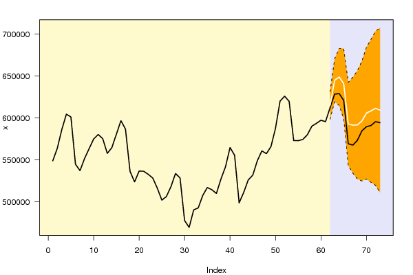
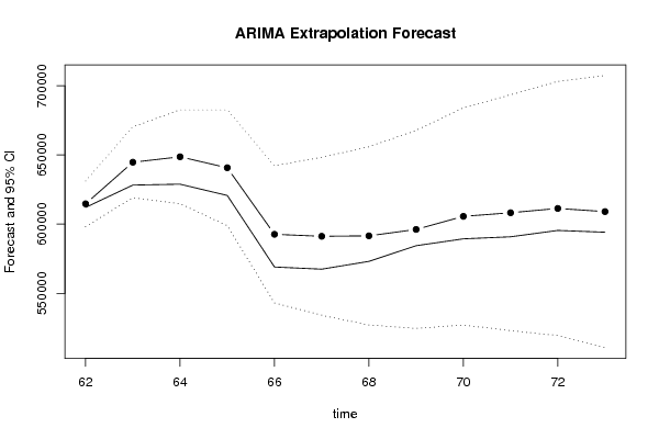
Title produced by software

ARIMA Forecasting

Date of computation

Wed, 22 Dec 2010 13:25:50 +0000

Cite this page as follows

Statistical Computations at FreeStatistics.org, Office for Research Development and Education, URL https://freestatistics.org/blog/index.php?v=date/2010/Dec/22/t12930242263lb4lscu519fyfr.htm/, Retrieved Sun, 05 May 2024 22:20:55 +0000

Statistical Computations at FreeStatistics.org, Office for Research Development and Education, URL https://freestatistics.org/blog/index.php?pk=114196, Retrieved Sun, 05 May 2024 22:20:55 +0000

QR Codes:

Paste this QR Code to cite your computation.

Original text written by user:

IsPrivate?

No (this computation is public)

User-defined keywords

Estimated Impact

128

Family? (F = Feedback message, R = changed R code, M = changed R Module, P = changed Parameters, D = changed Data)

-     [Standard Deviation-Mean Plot] [SMP prof bach] [2008-12-15 22:25:20] [bc937651ef42bf891200cf0e0edc7238]
- RM    [Variance Reduction Matrix] [VRM prof bach] [2008-12-15 22:31:00] [bc937651ef42bf891200cf0e0edc7238]
- RMP     [(Partial) Autocorrelation Function] [ARIMA Prof bach A...] [2008-12-15 22:38:57] [bc937651ef42bf891200cf0e0edc7238]
- RMP       [ARIMA Backward Selection] [Arima backward se...] [2008-12-19 17:26:16] [bc937651ef42bf891200cf0e0edc7238]
- RMP         [ARIMA Forecasting] [ARIMA forecast pr...] [2008-12-20 11:34:44] [bc937651ef42bf891200cf0e0edc7238]
-  MPD            [ARIMA Forecasting] [ARIMA Forecasting] [2010-12-22 13:25:50] [733bf75cb326fe693c93e834bfd34d22] [Current]
-    D              [ARIMA Forecasting] [ARIMA Forecasting] [2010-12-24 15:04:34] [616fb52b46273b7e6805de1e68b3a688] 

Feedback Forum

Post a new message

Dataseries X:

Download CSV

Histogram

Boxplots

Summary of computational transaction
Raw Input	view raw input (R code)
Raw Output	view raw output of R engine
Computing time	2 seconds
R Server	'Sir Ronald Aylmer Fisher' @ 193.190.124.24

\begin{tabular}{lllllllll}
\hline
Summary of computational transaction \tabularnewline
Raw Input & view raw input (R code)  \tabularnewline
Raw Output & view raw output of R engine  \tabularnewline
Computing time & 2 seconds \tabularnewline
R Server & 'Sir Ronald Aylmer Fisher' @ 193.190.124.24 \tabularnewline
\hline
\end{tabular}
%Source: https://freestatistics.org/blog/index.php?pk=114196&T=0

[TABLE]
[ROW][C]Summary of computational transaction[/C][/ROW]
[ROW][C]Raw Input[/C][C]view raw input (R code) [/C][/ROW]
[ROW][C]Raw Output[/C][C]view raw output of R engine [/C][/ROW]
[ROW][C]Computing time[/C][C]2 seconds[/C][/ROW]
[ROW][C]R Server[/C][C]'Sir Ronald Aylmer Fisher' @ 193.190.124.24[/C][/ROW]
[/TABLE]
Source: https://freestatistics.org/blog/index.php?pk=114196&T=0

Globally Unique Identifier (entire table): ba.freestatistics.org/blog/index.php?pk=114196&T=0

As an alternative you can also use a QR Code:

The GUIDs for individual cells are displayed in the table below:

Summary of computational transaction
Raw Input	view raw input (R code)
Raw Output	view raw output of R engine
Computing time	2 seconds
R Server	'Sir Ronald Aylmer Fisher' @ 193.190.124.24

Univariate ARIMA Extrapolation Forecast
time	Y[t]	F[t]	95% LB	95% UB	p-value(H0: Y[t] = F[t])	P(F[t]>Y[t-1])	P(F[t]>Y[t-s])	P(F[t]>Y[61])
49	565742	-	-	-	-	-	-	-
50	587625	-	-	-	-	-	-	-
51	619916	-	-	-	-	-	-	-
52	625809	-	-	-	-	-	-	-
53	619567	-	-	-	-	-	-	-
54	572942	-	-	-	-	-	-	-
55	572775	-	-	-	-	-	-	-
56	574205	-	-	-	-	-	-	-
57	579799	-	-	-	-	-	-	-
58	590072	-	-	-	-	-	-	-
59	593408	-	-	-	-	-	-	-
60	597141	-	-	-	-	-	-	-
61	595404	-	-	-	-	-	-	-
62	612117	614697.8118	598225.8938	631169.7298	0.3794	0.9892	0.9994	0.9892
63	628232	644742.7116	619172.4962	670312.927	0.1028	0.9938	0.9715	0.9999
64	628884	648687.2375	614801.6891	682572.7859	0.126	0.8816	0.9071	0.999
65	620735	640754.9516	598906.5047	682603.3985	0.1742	0.7109	0.8395	0.9832
66	569028	592663.642	543091.8737	642235.4103	0.175	0.1335	0.7822	0.4569
67	567456	591224.63	534133.8285	648315.4315	0.2072	0.777	0.7368	0.443
68	573100	591551.1697	527134.3466	655967.9929	0.2873	0.7683	0.7012	0.4533
69	584428	596187.9267	524634.4267	667741.4267	0.3737	0.7364	0.6733	0.5086
70	589379	605630.5259	527127.8999	684133.1519	0.3425	0.7017	0.6512	0.6008
71	590865	608246.1598	522979.9801	693512.3395	0.3447	0.6677	0.6335	0.6161
72	595454	611354.2479	519507.2674	703201.2285	0.3672	0.669	0.6192	0.6332
73	594167	609075.1419	510826.3489	707323.9348	0.3831	0.6071	0.6075	0.6075

\begin{tabular}{lllllllll}
\hline
Univariate ARIMA Extrapolation Forecast \tabularnewline
time & Y[t] & F[t] & 95% LB & 95% UB & p-value(H0: Y[t] = F[t]) & P(F[t]>Y[t-1]) & P(F[t]>Y[t-s]) & P(F[t]>Y[61]) \tabularnewline
49 & 565742 & - & - & - & - & - & - & - \tabularnewline
50 & 587625 & - & - & - & - & - & - & - \tabularnewline
51 & 619916 & - & - & - & - & - & - & - \tabularnewline
52 & 625809 & - & - & - & - & - & - & - \tabularnewline
53 & 619567 & - & - & - & - & - & - & - \tabularnewline
54 & 572942 & - & - & - & - & - & - & - \tabularnewline
55 & 572775 & - & - & - & - & - & - & - \tabularnewline
56 & 574205 & - & - & - & - & - & - & - \tabularnewline
57 & 579799 & - & - & - & - & - & - & - \tabularnewline
58 & 590072 & - & - & - & - & - & - & - \tabularnewline
59 & 593408 & - & - & - & - & - & - & - \tabularnewline
60 & 597141 & - & - & - & - & - & - & - \tabularnewline
61 & 595404 & - & - & - & - & - & - & - \tabularnewline
62 & 612117 & 614697.8118 & 598225.8938 & 631169.7298 & 0.3794 & 0.9892 & 0.9994 & 0.9892 \tabularnewline
63 & 628232 & 644742.7116 & 619172.4962 & 670312.927 & 0.1028 & 0.9938 & 0.9715 & 0.9999 \tabularnewline
64 & 628884 & 648687.2375 & 614801.6891 & 682572.7859 & 0.126 & 0.8816 & 0.9071 & 0.999 \tabularnewline
65 & 620735 & 640754.9516 & 598906.5047 & 682603.3985 & 0.1742 & 0.7109 & 0.8395 & 0.9832 \tabularnewline
66 & 569028 & 592663.642 & 543091.8737 & 642235.4103 & 0.175 & 0.1335 & 0.7822 & 0.4569 \tabularnewline
67 & 567456 & 591224.63 & 534133.8285 & 648315.4315 & 0.2072 & 0.777 & 0.7368 & 0.443 \tabularnewline
68 & 573100 & 591551.1697 & 527134.3466 & 655967.9929 & 0.2873 & 0.7683 & 0.7012 & 0.4533 \tabularnewline
69 & 584428 & 596187.9267 & 524634.4267 & 667741.4267 & 0.3737 & 0.7364 & 0.6733 & 0.5086 \tabularnewline
70 & 589379 & 605630.5259 & 527127.8999 & 684133.1519 & 0.3425 & 0.7017 & 0.6512 & 0.6008 \tabularnewline
71 & 590865 & 608246.1598 & 522979.9801 & 693512.3395 & 0.3447 & 0.6677 & 0.6335 & 0.6161 \tabularnewline
72 & 595454 & 611354.2479 & 519507.2674 & 703201.2285 & 0.3672 & 0.669 & 0.6192 & 0.6332 \tabularnewline
73 & 594167 & 609075.1419 & 510826.3489 & 707323.9348 & 0.3831 & 0.6071 & 0.6075 & 0.6075 \tabularnewline
\hline
\end{tabular}
%Source: https://freestatistics.org/blog/index.php?pk=114196&T=1

[TABLE]
[ROW][C]Univariate ARIMA Extrapolation Forecast[/C][/ROW]
[ROW][C]time[/C][C]Y[t][/C][C]F[t][/C][C]95% LB[/C][C]95% UB[/C][C]p-value(H0: Y[t] = F[t])[/C][C]P(F[t]>Y[t-1])[/C][C]P(F[t]>Y[t-s])[/C][C]P(F[t]>Y[61])[/C][/ROW]
[ROW][C]49[/C][C]565742[/C][C]-[/C][C]-[/C][C]-[/C][C]-[/C][C]-[/C][C]-[/C][C]-[/C][/ROW]
[ROW][C]50[/C][C]587625[/C][C]-[/C][C]-[/C][C]-[/C][C]-[/C][C]-[/C][C]-[/C][C]-[/C][/ROW]
[ROW][C]51[/C][C]619916[/C][C]-[/C][C]-[/C][C]-[/C][C]-[/C][C]-[/C][C]-[/C][C]-[/C][/ROW]
[ROW][C]52[/C][C]625809[/C][C]-[/C][C]-[/C][C]-[/C][C]-[/C][C]-[/C][C]-[/C][C]-[/C][/ROW]
[ROW][C]53[/C][C]619567[/C][C]-[/C][C]-[/C][C]-[/C][C]-[/C][C]-[/C][C]-[/C][C]-[/C][/ROW]
[ROW][C]54[/C][C]572942[/C][C]-[/C][C]-[/C][C]-[/C][C]-[/C][C]-[/C][C]-[/C][C]-[/C][/ROW]
[ROW][C]55[/C][C]572775[/C][C]-[/C][C]-[/C][C]-[/C][C]-[/C][C]-[/C][C]-[/C][C]-[/C][/ROW]
[ROW][C]56[/C][C]574205[/C][C]-[/C][C]-[/C][C]-[/C][C]-[/C][C]-[/C][C]-[/C][C]-[/C][/ROW]
[ROW][C]57[/C][C]579799[/C][C]-[/C][C]-[/C][C]-[/C][C]-[/C][C]-[/C][C]-[/C][C]-[/C][/ROW]
[ROW][C]58[/C][C]590072[/C][C]-[/C][C]-[/C][C]-[/C][C]-[/C][C]-[/C][C]-[/C][C]-[/C][/ROW]
[ROW][C]59[/C][C]593408[/C][C]-[/C][C]-[/C][C]-[/C][C]-[/C][C]-[/C][C]-[/C][C]-[/C][/ROW]
[ROW][C]60[/C][C]597141[/C][C]-[/C][C]-[/C][C]-[/C][C]-[/C][C]-[/C][C]-[/C][C]-[/C][/ROW]
[ROW][C]61[/C][C]595404[/C][C]-[/C][C]-[/C][C]-[/C][C]-[/C][C]-[/C][C]-[/C][C]-[/C][/ROW]
[ROW][C]62[/C][C]612117[/C][C]614697.8118[/C][C]598225.8938[/C][C]631169.7298[/C][C]0.3794[/C][C]0.9892[/C][C]0.9994[/C][C]0.9892[/C][/ROW]
[ROW][C]63[/C][C]628232[/C][C]644742.7116[/C][C]619172.4962[/C][C]670312.927[/C][C]0.1028[/C][C]0.9938[/C][C]0.9715[/C][C]0.9999[/C][/ROW]
[ROW][C]64[/C][C]628884[/C][C]648687.2375[/C][C]614801.6891[/C][C]682572.7859[/C][C]0.126[/C][C]0.8816[/C][C]0.9071[/C][C]0.999[/C][/ROW]
[ROW][C]65[/C][C]620735[/C][C]640754.9516[/C][C]598906.5047[/C][C]682603.3985[/C][C]0.1742[/C][C]0.7109[/C][C]0.8395[/C][C]0.9832[/C][/ROW]
[ROW][C]66[/C][C]569028[/C][C]592663.642[/C][C]543091.8737[/C][C]642235.4103[/C][C]0.175[/C][C]0.1335[/C][C]0.7822[/C][C]0.4569[/C][/ROW]
[ROW][C]67[/C][C]567456[/C][C]591224.63[/C][C]534133.8285[/C][C]648315.4315[/C][C]0.2072[/C][C]0.777[/C][C]0.7368[/C][C]0.443[/C][/ROW]
[ROW][C]68[/C][C]573100[/C][C]591551.1697[/C][C]527134.3466[/C][C]655967.9929[/C][C]0.2873[/C][C]0.7683[/C][C]0.7012[/C][C]0.4533[/C][/ROW]
[ROW][C]69[/C][C]584428[/C][C]596187.9267[/C][C]524634.4267[/C][C]667741.4267[/C][C]0.3737[/C][C]0.7364[/C][C]0.6733[/C][C]0.5086[/C][/ROW]
[ROW][C]70[/C][C]589379[/C][C]605630.5259[/C][C]527127.8999[/C][C]684133.1519[/C][C]0.3425[/C][C]0.7017[/C][C]0.6512[/C][C]0.6008[/C][/ROW]
[ROW][C]71[/C][C]590865[/C][C]608246.1598[/C][C]522979.9801[/C][C]693512.3395[/C][C]0.3447[/C][C]0.6677[/C][C]0.6335[/C][C]0.6161[/C][/ROW]
[ROW][C]72[/C][C]595454[/C][C]611354.2479[/C][C]519507.2674[/C][C]703201.2285[/C][C]0.3672[/C][C]0.669[/C][C]0.6192[/C][C]0.6332[/C][/ROW]
[ROW][C]73[/C][C]594167[/C][C]609075.1419[/C][C]510826.3489[/C][C]707323.9348[/C][C]0.3831[/C][C]0.6071[/C][C]0.6075[/C][C]0.6075[/C][/ROW]
[/TABLE]
Source: https://freestatistics.org/blog/index.php?pk=114196&T=1

Globally Unique Identifier (entire table): ba.freestatistics.org/blog/index.php?pk=114196&T=1

As an alternative you can also use a QR Code:

The GUIDs for individual cells are displayed in the table below:

Univariate ARIMA Extrapolation Forecast
time	Y[t]	F[t]	95% LB	95% UB	p-value(H0: Y[t] = F[t])	P(F[t]>Y[t-1])	P(F[t]>Y[t-s])	P(F[t]>Y[61])
49	565742	-	-	-	-	-	-	-
50	587625	-	-	-	-	-	-	-
51	619916	-	-	-	-	-	-	-
52	625809	-	-	-	-	-	-	-
53	619567	-	-	-	-	-	-	-
54	572942	-	-	-	-	-	-	-
55	572775	-	-	-	-	-	-	-
56	574205	-	-	-	-	-	-	-
57	579799	-	-	-	-	-	-	-
58	590072	-	-	-	-	-	-	-
59	593408	-	-	-	-	-	-	-
60	597141	-	-	-	-	-	-	-
61	595404	-	-	-	-	-	-	-
62	612117	614697.8118	598225.8938	631169.7298	0.3794	0.9892	0.9994	0.9892
63	628232	644742.7116	619172.4962	670312.927	0.1028	0.9938	0.9715	0.9999
64	628884	648687.2375	614801.6891	682572.7859	0.126	0.8816	0.9071	0.999
65	620735	640754.9516	598906.5047	682603.3985	0.1742	0.7109	0.8395	0.9832
66	569028	592663.642	543091.8737	642235.4103	0.175	0.1335	0.7822	0.4569
67	567456	591224.63	534133.8285	648315.4315	0.2072	0.777	0.7368	0.443
68	573100	591551.1697	527134.3466	655967.9929	0.2873	0.7683	0.7012	0.4533
69	584428	596187.9267	524634.4267	667741.4267	0.3737	0.7364	0.6733	0.5086
70	589379	605630.5259	527127.8999	684133.1519	0.3425	0.7017	0.6512	0.6008
71	590865	608246.1598	522979.9801	693512.3395	0.3447	0.6677	0.6335	0.6161
72	595454	611354.2479	519507.2674	703201.2285	0.3672	0.669	0.6192	0.6332
73	594167	609075.1419	510826.3489	707323.9348	0.3831	0.6071	0.6075	0.6075

Univariate ARIMA Extrapolation Forecast Performance
time	% S.E.	PE	MAPE	Sq.E	MSE	RMSE
62	0.0137	-0.0042	3e-04	6660589.6831	555049.1403	745.0162
63	0.0202	-0.0256	0.0021	272603597.7043	22716966.4754	4766.2319
64	0.0267	-0.0305	0.0025	392168214.0299	32680684.5025	5716.7022
65	0.0333	-0.0312	0.0026	400798461.5498	33399871.7958	5779.2622
66	0.0427	-0.0399	0.0033	558643572.0411	46553631.0034	6823.0221
67	0.0493	-0.0402	0.0034	564947773.2936	47078981.1078	6861.4125
68	0.0556	-0.0312	0.0026	340445664.462	28370472.0385	5326.3939
69	0.0612	-0.0197	0.0016	138295875.3157	11524656.2763	3394.7984
70	0.0661	-0.0268	0.0022	264112094.1694	22009341.1808	4691.4114
71	0.0715	-0.0286	0.0024	302104716.584	25175393.0487	5017.5086
72	0.0767	-0.026	0.0022	252817884.759	21068157.0632	4590.0062
73	0.0823	-0.0245	0.002	222252693.4554	18521057.7879	4303.6099

\begin{tabular}{lllllllll}
\hline
Univariate ARIMA Extrapolation Forecast Performance \tabularnewline
time & % S.E. & PE & MAPE & Sq.E & MSE & RMSE \tabularnewline
62 & 0.0137 & -0.0042 & 3e-04 & 6660589.6831 & 555049.1403 & 745.0162 \tabularnewline
63 & 0.0202 & -0.0256 & 0.0021 & 272603597.7043 & 22716966.4754 & 4766.2319 \tabularnewline
64 & 0.0267 & -0.0305 & 0.0025 & 392168214.0299 & 32680684.5025 & 5716.7022 \tabularnewline
65 & 0.0333 & -0.0312 & 0.0026 & 400798461.5498 & 33399871.7958 & 5779.2622 \tabularnewline
66 & 0.0427 & -0.0399 & 0.0033 & 558643572.0411 & 46553631.0034 & 6823.0221 \tabularnewline
67 & 0.0493 & -0.0402 & 0.0034 & 564947773.2936 & 47078981.1078 & 6861.4125 \tabularnewline
68 & 0.0556 & -0.0312 & 0.0026 & 340445664.462 & 28370472.0385 & 5326.3939 \tabularnewline
69 & 0.0612 & -0.0197 & 0.0016 & 138295875.3157 & 11524656.2763 & 3394.7984 \tabularnewline
70 & 0.0661 & -0.0268 & 0.0022 & 264112094.1694 & 22009341.1808 & 4691.4114 \tabularnewline
71 & 0.0715 & -0.0286 & 0.0024 & 302104716.584 & 25175393.0487 & 5017.5086 \tabularnewline
72 & 0.0767 & -0.026 & 0.0022 & 252817884.759 & 21068157.0632 & 4590.0062 \tabularnewline
73 & 0.0823 & -0.0245 & 0.002 & 222252693.4554 & 18521057.7879 & 4303.6099 \tabularnewline
\hline
\end{tabular}
%Source: https://freestatistics.org/blog/index.php?pk=114196&T=2

[TABLE]
[ROW][C]Univariate ARIMA Extrapolation Forecast Performance[/C][/ROW]
[ROW][C]time[/C][C]% S.E.[/C][C]PE[/C][C]MAPE[/C][C]Sq.E[/C][C]MSE[/C][C]RMSE[/C][/ROW]
[ROW][C]62[/C][C]0.0137[/C][C]-0.0042[/C][C]3e-04[/C][C]6660589.6831[/C][C]555049.1403[/C][C]745.0162[/C][/ROW]
[ROW][C]63[/C][C]0.0202[/C][C]-0.0256[/C][C]0.0021[/C][C]272603597.7043[/C][C]22716966.4754[/C][C]4766.2319[/C][/ROW]
[ROW][C]64[/C][C]0.0267[/C][C]-0.0305[/C][C]0.0025[/C][C]392168214.0299[/C][C]32680684.5025[/C][C]5716.7022[/C][/ROW]
[ROW][C]65[/C][C]0.0333[/C][C]-0.0312[/C][C]0.0026[/C][C]400798461.5498[/C][C]33399871.7958[/C][C]5779.2622[/C][/ROW]
[ROW][C]66[/C][C]0.0427[/C][C]-0.0399[/C][C]0.0033[/C][C]558643572.0411[/C][C]46553631.0034[/C][C]6823.0221[/C][/ROW]
[ROW][C]67[/C][C]0.0493[/C][C]-0.0402[/C][C]0.0034[/C][C]564947773.2936[/C][C]47078981.1078[/C][C]6861.4125[/C][/ROW]
[ROW][C]68[/C][C]0.0556[/C][C]-0.0312[/C][C]0.0026[/C][C]340445664.462[/C][C]28370472.0385[/C][C]5326.3939[/C][/ROW]
[ROW][C]69[/C][C]0.0612[/C][C]-0.0197[/C][C]0.0016[/C][C]138295875.3157[/C][C]11524656.2763[/C][C]3394.7984[/C][/ROW]
[ROW][C]70[/C][C]0.0661[/C][C]-0.0268[/C][C]0.0022[/C][C]264112094.1694[/C][C]22009341.1808[/C][C]4691.4114[/C][/ROW]
[ROW][C]71[/C][C]0.0715[/C][C]-0.0286[/C][C]0.0024[/C][C]302104716.584[/C][C]25175393.0487[/C][C]5017.5086[/C][/ROW]
[ROW][C]72[/C][C]0.0767[/C][C]-0.026[/C][C]0.0022[/C][C]252817884.759[/C][C]21068157.0632[/C][C]4590.0062[/C][/ROW]
[ROW][C]73[/C][C]0.0823[/C][C]-0.0245[/C][C]0.002[/C][C]222252693.4554[/C][C]18521057.7879[/C][C]4303.6099[/C][/ROW]
[/TABLE]
Source: https://freestatistics.org/blog/index.php?pk=114196&T=2

Globally Unique Identifier (entire table): ba.freestatistics.org/blog/index.php?pk=114196&T=2

As an alternative you can also use a QR Code:

The GUIDs for individual cells are displayed in the table below:

Univariate ARIMA Extrapolation Forecast Performance
time	% S.E.	PE	MAPE	Sq.E	MSE	RMSE
62	0.0137	-0.0042	3e-04	6660589.6831	555049.1403	745.0162
63	0.0202	-0.0256	0.0021	272603597.7043	22716966.4754	4766.2319
64	0.0267	-0.0305	0.0025	392168214.0299	32680684.5025	5716.7022
65	0.0333	-0.0312	0.0026	400798461.5498	33399871.7958	5779.2622
66	0.0427	-0.0399	0.0033	558643572.0411	46553631.0034	6823.0221
67	0.0493	-0.0402	0.0034	564947773.2936	47078981.1078	6861.4125
68	0.0556	-0.0312	0.0026	340445664.462	28370472.0385	5326.3939
69	0.0612	-0.0197	0.0016	138295875.3157	11524656.2763	3394.7984
70	0.0661	-0.0268	0.0022	264112094.1694	22009341.1808	4691.4114
71	0.0715	-0.0286	0.0024	302104716.584	25175393.0487	5017.5086
72	0.0767	-0.026	0.0022	252817884.759	21068157.0632	4590.0062
73	0.0823	-0.0245	0.002	222252693.4554	18521057.7879	4303.6099

Figure 1

PNG link

Postscript link

PDF link

Figure 2

PNG link

Postscript link

PDF link

Parameters (Session):

par1 = 12 ; par2 = 1 ; par3 = 1 ; par4 = 1 ; par5 = 12 ; par6 = 1 ; par7 = 1 ; par8 = 0 ; par9 = 0 ; par10 = FALSE ;

Parameters (R input):

par1 = 12 ; par2 = 1 ; par3 = 1 ; par4 = 1 ; par5 = 12 ; par6 = 1 ; par7 = 1 ; par8 = 0 ; par9 = 0 ; par10 = FALSE ;

R code (references can be found in the software module):

par1 <- as.numeric(par1) #cut off periods
par2 <- as.numeric(par2) #lambda
par3 <- as.numeric(par3) #degree of non-seasonal differencing
par4 <- as.numeric(par4) #degree of seasonal differencing
par5 <- as.numeric(par5) #seasonal period
par6 <- as.numeric(par6) #p
par7 <- as.numeric(par7) #q
par8 <- as.numeric(par8) #P
par9 <- as.numeric(par9) #Q
if (par10 == 'TRUE') par10 <- TRUE
if (par10 == 'FALSE') par10 <- FALSE
if (par2 == 0) x <- log(x)
if (par2 != 0) x <- x^par2
lx <- length(x)
first <- lx - 2*par1
nx <- lx - par1
nx1 <- nx + 1
fx <- lx - nx
if (fx < 1) {
fx <- par5
nx1 <- lx + fx - 1
first <- lx - 2*fx
}
first <- 1
if (fx < 3) fx <- round(lx/10,0)
(arima.out <- arima(x[1:nx], order=c(par6,par3,par7), seasonal=list(order=c(par8,par4,par9), period=par5), include.mean=par10, method='ML'))
(forecast <- predict(arima.out,fx))
(lb <- forecast$pred - 1.96 * forecast$se)
(ub <- forecast$pred + 1.96 * forecast$se)
if (par2 == 0) {
x <- exp(x)
forecast$pred <- exp(forecast$pred)
lb <- exp(lb)
ub <- exp(ub)
}
if (par2 != 0) {
x <- x^(1/par2)
forecast$pred <- forecast$pred^(1/par2)
lb <- lb^(1/par2)
ub <- ub^(1/par2)
}
if (par2 < 0) {
olb <- lb
lb <- ub
ub <- olb
}
(actandfor <- c(x[1:nx], forecast$pred))
(perc.se <- (ub-forecast$pred)/1.96/forecast$pred)
bitmap(file='test1.png')
opar <- par(mar=c(4,4,2,2),las=1)
ylim <- c( min(x[first:nx],lb), max(x[first:nx],ub))
plot(x,ylim=ylim,type='n',xlim=c(first,lx))
usr <- par('usr')
rect(usr[1],usr[3],nx+1,usr[4],border=NA,col='lemonchiffon')
rect(nx1,usr[3],usr[2],usr[4],border=NA,col='lavender')
abline(h= (-3:3)*2 , col ='gray', lty =3)
polygon( c(nx1:lx,lx:nx1), c(lb,rev(ub)), col = 'orange', lty=2,border=NA)
lines(nx1:lx, lb , lty=2)
lines(nx1:lx, ub , lty=2)
lines(x, lwd=2)
lines(nx1:lx, forecast$pred , lwd=2 , col ='white')
box()
par(opar)
dev.off()
prob.dec <- array(NA, dim=fx)
prob.sdec <- array(NA, dim=fx)
prob.ldec <- array(NA, dim=fx)
prob.pval <- array(NA, dim=fx)
perf.pe <- array(0, dim=fx)
perf.mape <- array(0, dim=fx)
perf.se <- array(0, dim=fx)
perf.mse <- array(0, dim=fx)
perf.rmse <- array(0, dim=fx)
for (i in 1:fx) {
locSD <- (ub[i] - forecast$pred[i]) / 1.96
perf.pe[i] = (x[nx+i] - forecast$pred[i]) / forecast$pred[i]
perf.mape[i] = perf.mape[i] + abs(perf.pe[i])
perf.se[i] = (x[nx+i] - forecast$pred[i])^2
perf.mse[i] = perf.mse[i] + perf.se[i]
prob.dec[i] = pnorm((x[nx+i-1] - forecast$pred[i]) / locSD)
prob.sdec[i] = pnorm((x[nx+i-par5] - forecast$pred[i]) / locSD)
prob.ldec[i] = pnorm((x[nx] - forecast$pred[i]) / locSD)
prob.pval[i] = pnorm(abs(x[nx+i] - forecast$pred[i]) / locSD)
}
perf.mape = perf.mape / fx
perf.mse = perf.mse / fx
perf.rmse = sqrt(perf.mse)
bitmap(file='test2.png')
plot(forecast$pred, pch=19, type='b',main='ARIMA Extrapolation Forecast', ylab='Forecast and 95% CI', xlab='time',ylim=c(min(lb),max(ub)))
dum <- forecast$pred
dum[1:12] <- x[(nx+1):lx]
lines(dum, lty=1)
lines(ub,lty=3)
lines(lb,lty=3)
dev.off()
load(file='createtable')
a<-table.start()
a<-table.row.start(a)
a<-table.element(a,'Univariate ARIMA Extrapolation Forecast',9,TRUE)
a<-table.row.end(a)
a<-table.row.start(a)
a<-table.element(a,'time',1,header=TRUE)
a<-table.element(a,'Y[t]',1,header=TRUE)
a<-table.element(a,'F[t]',1,header=TRUE)
a<-table.element(a,'95% LB',1,header=TRUE)
a<-table.element(a,'95% UB',1,header=TRUE)
a<-table.element(a,'p-value
(H0: Y[t] = F[t])',1,header=TRUE)
a<-table.element(a,'P(F[t]>Y[t-1])',1,header=TRUE)
a<-table.element(a,'P(F[t]>Y[t-s])',1,header=TRUE)
mylab <- paste('P(F[t]>Y[',nx,sep='')
mylab <- paste(mylab,'])',sep='')
a<-table.element(a,mylab,1,header=TRUE)
a<-table.row.end(a)
for (i in (nx-par5):nx) {
a<-table.row.start(a)
a<-table.element(a,i,header=TRUE)
a<-table.element(a,x[i])
a<-table.element(a,'-')
a<-table.element(a,'-')
a<-table.element(a,'-')
a<-table.element(a,'-')
a<-table.element(a,'-')
a<-table.element(a,'-')
a<-table.element(a,'-')
a<-table.row.end(a)
}
for (i in 1:fx) {
a<-table.row.start(a)
a<-table.element(a,nx+i,header=TRUE)
a<-table.element(a,round(x[nx+i],4))
a<-table.element(a,round(forecast$pred[i],4))
a<-table.element(a,round(lb[i],4))
a<-table.element(a,round(ub[i],4))
a<-table.element(a,round((1-prob.pval[i]),4))
a<-table.element(a,round((1-prob.dec[i]),4))
a<-table.element(a,round((1-prob.sdec[i]),4))
a<-table.element(a,round((1-prob.ldec[i]),4))
a<-table.row.end(a)
}
a<-table.end(a)
table.save(a,file='mytable.tab')
a<-table.start()
a<-table.row.start(a)
a<-table.element(a,'Univariate ARIMA Extrapolation Forecast Performance',7,TRUE)
a<-table.row.end(a)
a<-table.row.start(a)
a<-table.element(a,'time',1,header=TRUE)
a<-table.element(a,'% S.E.',1,header=TRUE)
a<-table.element(a,'PE',1,header=TRUE)
a<-table.element(a,'MAPE',1,header=TRUE)
a<-table.element(a,'Sq.E',1,header=TRUE)
a<-table.element(a,'MSE',1,header=TRUE)
a<-table.element(a,'RMSE',1,header=TRUE)
a<-table.row.end(a)
for (i in 1:fx) {
a<-table.row.start(a)
a<-table.element(a,nx+i,header=TRUE)
a<-table.element(a,round(perc.se[i],4))
a<-table.element(a,round(perf.pe[i],4))
a<-table.element(a,round(perf.mape[i],4))
a<-table.element(a,round(perf.se[i],4))
a<-table.element(a,round(perf.mse[i],4))
a<-table.element(a,round(perf.rmse[i],4))
a<-table.row.end(a)
}
a<-table.end(a)
table.save(a,file='mytable1.tab')

Free Statistics

Description of Statistical Computation

Tree of Dependent Computations

Dataset

Tables (Output of Computation)

Figures (Output of Computation)

Input Parameters & R Code