Free Statistics

of Irreproducible Research!

Author's title

Author*The author of this computation has been verified*
R Software Modulerwasp_arimaforecasting.wasp
Title produced by softwareARIMA Forecasting
Date of computationMon, 20 Dec 2010 23:26:43 +0000
Cite this page as followsStatistical Computations at FreeStatistics.org, Office for Research Development and Education, URL https://freestatistics.org/blog/index.php?v=date/2010/Dec/21/t129288747918dr8xto30vk4r0.htm/, Retrieved Sun, 19 May 2024 17:11:50 +0000
Statistical Computations at FreeStatistics.org, Office for Research Development and Education, URL https://freestatistics.org/blog/index.php?pk=113170, Retrieved Sun, 19 May 2024 17:11:50 +0000
QR Codes:

Original text written by user:
IsPrivate?No (this computation is public)
User-defined keywords
Estimated Impact147
Family? (F = Feedback message, R = changed R code, M = changed R Module, P = changed Parameters, D = changed Data)
-     [Univariate Data Series] [data set] [2008-12-01 19:54:57] [b98453cac15ba1066b407e146608df68]
- RMP   [Standard Deviation-Mean Plot] [Unemployment] [2010-11-29 10:34:47] [b98453cac15ba1066b407e146608df68]
- RMP     [ARIMA Forecasting] [Unemployment] [2010-11-29 20:46:45] [b98453cac15ba1066b407e146608df68]
- R PD        [ARIMA Forecasting] [Voorspelling Doll...] [2010-12-20 23:26:43] [109f5cd2d2b7c934778912c55604f6f1] [Current]
Feedback Forum

Post a new message
Dataseries X:
1,3866
1,3582
1,3332
1,3595
1,3617
1,3684
1,3394
1,3262
1,3173
1,3085
1,327
1,3182
1,293
1,291
1,2984
1,2795
1,299
1,3174
1,326
1,3111
1,2816
1,276
1,2849
1,2818
1,2829
1,2796
1,3008
1,2967
1,2938
1,2833
1,2823
1,2765
1,2634
1,2596
1,2705
1,2591
1,2798
1,2763
1,2795
1,2782
1,2644
1,2596
1,2615
1,2555
1,2555
1,2658
1,2565
1,2783
1,2786
1,2782
1,2905
1,3042
1,2942
1,313
1,3671
1,3549
1,3558
1,3507
1,3494
1,3607
1,3295
1,3193
1,3308
1,3246
1,3392
1,3425
1,3496
1,3255
1,3231
1,3273
1,3276
1,3173
1,3196
1,3058
1,2966
1,2932
1,2947
1,305
1,3232
1,3125
1,2992
1,3266
1,3275
1,3223
1,3403
1,3322
1,3363
1,3425
1,3574
1,3683
1,3623
1,3563
1,3518
1,3494
1,3612
1,369
1,3771
1,3972
1,401
1,3908
1,3901
1,3856
1,4098
1,422
1,4238
1,4207
1,4095
1,4177
1,3866
1,3959
1,4102
1,3969
1,4004
1,385
1,389
1,384
1,392
1,3932
1,3858
1,3978
1,4029
1,394
1,4096
1,4058
1,4134
1,4096
1,4049
1,4009
1,3897
1,4019
1,3901
1,399
1,3901
1,3975
1,3991
1,4089
1,413
1,409
1,4217
1,4223
1,4191
1,4229
1,4227
1,4269
1,4229
1,4104
1,4053
1,4138
1,4303
1,4384
1,441
1,437
1,4357
1,4202
1,4166
1,417
1,4293
1,4294
1,4072
1,4101
1,4112
1,4243
1,433
1,4323
1,4324
1,427
1,4268
1,4364
1,4272
1,4314
1,422
1,4335
1,4262
1,433
1,4473
1,4522
1,4545
1,4594
1,4561
1,4611
1,4671
1,4712
1,4705
1,4658
1,478
1,4783
1,4768
1,467
1,465
1,4549
1,4643
1,4539
1,4537
1,4616
1,4722
1,4694
1,4763
1,475
1,4765
1,4864
1,4881
1,4864
1,4869
1,4918
1,4971
1,4921
1,5
1,502
1,5019
1,4874
1,4785
1,4788
1,48
1,4772
1,4658
1,4761
1,4867
1,4862
1,4984
1,4966
1,5037
1,4922
1,4868
1,4965
1,4875
1,4957
1,4863
1,4815
1,4968
1,4969
1,5083
1,5071
1,4918
1,5023
1,5074
1,509
1,512
1,5068
1,4787
1,4774
1,4768
1,473
1,4757
1,4647
1,4541
1,456
1,4343
1,4337
1,4368
1,4279
1,4276
1,4398
1,4405
1,4433
1,4338
1,4406
1,4389
1,4442
1,435
1,4304
1,4273
1,4528
1,4481
1,4563
1,4486
1,4374
1,4369
1,4279
1,4132
1,4064
1,4135
1,4151
1,4085
1,4072
1,3999
1,3966
1,3913
1,3937
1,3984
1,3847
1,3691
1,3675
1,376
1,374
1,3718
1,3572
1,3607
1,3649
1,3726
1,3567
1,3519
1,3626
1,3577
1,3547
1,3489
1,357
1,3525
1,3548
1,3641
1,3668
1,3582
1,3662
1,3557
1,361
1,3657
1,3765
1,3705
1,3723
1,3756
1,366
1,3548
1,3471
1,3519
1,3338
1,3356
1,3353
1,3471
1,3482
1,3479
1,3468
1,3396
1,334
1,3296
1,3384
1,3585
1,3583
1,3615
1,3544
1,3535
1,3432
1,3486
1,3373
1,3339
1,3311
1,3321
1,329
1,3245
1,3256
1,3315
1,3238
1,3089
1,2924
1,2727
1,2746
1,2969
1,2698
1,2686
1,2587
1,2492
1,2349
1,2428
1,227
1,2334
1,2497
1,236
1,2223
1,2309
1,2255
1,2384
1,2307
1,2155
1,2218
1,2268
1,206
1,1959
1,1942


Summary of computational transaction
Raw Inputview raw input (R code)
Raw Outputview raw output of R engine
Computing time2 seconds
R Server'Gwilym Jenkins' @ 72.249.127.135

\begin{tabular}{lllllllll}
\hline
Summary of computational transaction \tabularnewline
Raw Input & view raw input (R code)  \tabularnewline
Raw Output & view raw output of R engine  \tabularnewline
Computing time & 2 seconds \tabularnewline
R Server & 'Gwilym Jenkins' @ 72.249.127.135 \tabularnewline
\hline
\end{tabular}
%Source: https://freestatistics.org/blog/index.php?pk=113170&T=0

[TABLE]
[ROW][C]Summary of computational transaction[/C][/ROW]
[ROW][C]Raw Input[/C][C]view raw input (R code) [/C][/ROW]
[ROW][C]Raw Output[/C][C]view raw output of R engine [/C][/ROW]
[ROW][C]Computing time[/C][C]2 seconds[/C][/ROW]
[ROW][C]R Server[/C][C]'Gwilym Jenkins' @ 72.249.127.135[/C][/ROW]
[/TABLE]
Source: https://freestatistics.org/blog/index.php?pk=113170&T=0

Globally Unique Identifier (entire table): ba.freestatistics.org/blog/index.php?pk=113170&T=0

As an alternative you can also use a QR Code:  

The GUIDs for individual cells are displayed in the table below:

Summary of computational transaction
Raw Inputview raw input (R code)
Raw Outputview raw output of R engine
Computing time2 seconds
R Server'Gwilym Jenkins' @ 72.249.127.135


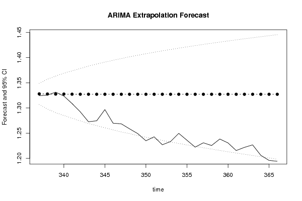
Univariate ARIMA Extrapolation Forecast
timeY[t]F[t]95% LB95% UBp-value(H0: Y[t] = F[t])P(F[t]>Y[t-1])P(F[t]>Y[t-s])P(F[t]>Y[336])
3311.3486-------
3321.3373-------
3331.3339-------
3341.3311-------
3351.3321-------
3361.329-------
3371.32451.32811.3071.34890.36770.46590.19310.4659
3381.32561.32781.29781.35720.44120.58760.34250.4686
3391.33151.32761.29081.36350.41560.54340.42410.4694
3401.32381.32771.28511.36910.42720.42810.4170.475
3411.30891.32741.27971.37360.21590.56110.47340.4734
3421.29241.32741.27431.37860.09050.760.54350.4749
3431.27271.32731.26941.38310.02740.89020.52430.4766
3441.27461.32731.26481.38730.04240.96290.44560.478
3451.29691.32731.26061.39120.17520.94720.5430.4795
3461.26981.32731.25651.39480.04750.81130.70340.4803
3471.26861.32731.25271.39830.05260.94370.83220.4812
3481.25871.32731.2491.40160.03530.93910.9250.4821
3491.24921.32731.24551.40480.02420.95860.90860.4828
3501.23491.32731.24211.40780.01230.97130.77020.4834
3511.24281.32731.23881.41080.02360.9850.91150.484
3521.2271.32731.23561.41360.01140.97250.90880.4845
3531.23341.32731.23261.41630.01930.98640.93450.485
3541.24971.32731.22961.41890.04850.97770.95260.4854
3551.2361.32731.22671.42150.02870.94680.97270.4858
3561.22231.32731.22381.4240.01660.96790.95660.4862
3571.23091.32731.2211.42640.02830.98110.97640.4865
3581.22551.32731.21831.42870.02460.96870.96520.4868
3591.23841.32731.21571.4310.04650.97280.92870.4871
3601.23071.32731.21311.43330.0370.94990.95440.4874
3611.21551.32731.21061.43540.02140.960.97150.4876
3621.22181.32731.20811.43760.03040.97650.95670.4879
3631.22681.32731.20561.43970.03980.96710.96210.4881
3641.2061.32731.20321.44170.01890.95740.93610.4883
3651.19591.32731.20081.44370.01350.97940.9480.4885
3661.19421.32731.19851.44570.01380.98520.96790.4887

\begin{tabular}{lllllllll}
\hline
Univariate ARIMA Extrapolation Forecast \tabularnewline
time & Y[t] & F[t] & 95% LB & 95% UB & p-value(H0: Y[t] = F[t]) & P(F[t]>Y[t-1]) & P(F[t]>Y[t-s]) & P(F[t]>Y[336]) \tabularnewline
331 & 1.3486 & - & - & - & - & - & - & - \tabularnewline
332 & 1.3373 & - & - & - & - & - & - & - \tabularnewline
333 & 1.3339 & - & - & - & - & - & - & - \tabularnewline
334 & 1.3311 & - & - & - & - & - & - & - \tabularnewline
335 & 1.3321 & - & - & - & - & - & - & - \tabularnewline
336 & 1.329 & - & - & - & - & - & - & - \tabularnewline
337 & 1.3245 & 1.3281 & 1.307 & 1.3489 & 0.3677 & 0.4659 & 0.1931 & 0.4659 \tabularnewline
338 & 1.3256 & 1.3278 & 1.2978 & 1.3572 & 0.4412 & 0.5876 & 0.3425 & 0.4686 \tabularnewline
339 & 1.3315 & 1.3276 & 1.2908 & 1.3635 & 0.4156 & 0.5434 & 0.4241 & 0.4694 \tabularnewline
340 & 1.3238 & 1.3277 & 1.2851 & 1.3691 & 0.4272 & 0.4281 & 0.417 & 0.475 \tabularnewline
341 & 1.3089 & 1.3274 & 1.2797 & 1.3736 & 0.2159 & 0.5611 & 0.4734 & 0.4734 \tabularnewline
342 & 1.2924 & 1.3274 & 1.2743 & 1.3786 & 0.0905 & 0.76 & 0.5435 & 0.4749 \tabularnewline
343 & 1.2727 & 1.3273 & 1.2694 & 1.3831 & 0.0274 & 0.8902 & 0.5243 & 0.4766 \tabularnewline
344 & 1.2746 & 1.3273 & 1.2648 & 1.3873 & 0.0424 & 0.9629 & 0.4456 & 0.478 \tabularnewline
345 & 1.2969 & 1.3273 & 1.2606 & 1.3912 & 0.1752 & 0.9472 & 0.543 & 0.4795 \tabularnewline
346 & 1.2698 & 1.3273 & 1.2565 & 1.3948 & 0.0475 & 0.8113 & 0.7034 & 0.4803 \tabularnewline
347 & 1.2686 & 1.3273 & 1.2527 & 1.3983 & 0.0526 & 0.9437 & 0.8322 & 0.4812 \tabularnewline
348 & 1.2587 & 1.3273 & 1.249 & 1.4016 & 0.0353 & 0.9391 & 0.925 & 0.4821 \tabularnewline
349 & 1.2492 & 1.3273 & 1.2455 & 1.4048 & 0.0242 & 0.9586 & 0.9086 & 0.4828 \tabularnewline
350 & 1.2349 & 1.3273 & 1.2421 & 1.4078 & 0.0123 & 0.9713 & 0.7702 & 0.4834 \tabularnewline
351 & 1.2428 & 1.3273 & 1.2388 & 1.4108 & 0.0236 & 0.985 & 0.9115 & 0.484 \tabularnewline
352 & 1.227 & 1.3273 & 1.2356 & 1.4136 & 0.0114 & 0.9725 & 0.9088 & 0.4845 \tabularnewline
353 & 1.2334 & 1.3273 & 1.2326 & 1.4163 & 0.0193 & 0.9864 & 0.9345 & 0.485 \tabularnewline
354 & 1.2497 & 1.3273 & 1.2296 & 1.4189 & 0.0485 & 0.9777 & 0.9526 & 0.4854 \tabularnewline
355 & 1.236 & 1.3273 & 1.2267 & 1.4215 & 0.0287 & 0.9468 & 0.9727 & 0.4858 \tabularnewline
356 & 1.2223 & 1.3273 & 1.2238 & 1.424 & 0.0166 & 0.9679 & 0.9566 & 0.4862 \tabularnewline
357 & 1.2309 & 1.3273 & 1.221 & 1.4264 & 0.0283 & 0.9811 & 0.9764 & 0.4865 \tabularnewline
358 & 1.2255 & 1.3273 & 1.2183 & 1.4287 & 0.0246 & 0.9687 & 0.9652 & 0.4868 \tabularnewline
359 & 1.2384 & 1.3273 & 1.2157 & 1.431 & 0.0465 & 0.9728 & 0.9287 & 0.4871 \tabularnewline
360 & 1.2307 & 1.3273 & 1.2131 & 1.4333 & 0.037 & 0.9499 & 0.9544 & 0.4874 \tabularnewline
361 & 1.2155 & 1.3273 & 1.2106 & 1.4354 & 0.0214 & 0.96 & 0.9715 & 0.4876 \tabularnewline
362 & 1.2218 & 1.3273 & 1.2081 & 1.4376 & 0.0304 & 0.9765 & 0.9567 & 0.4879 \tabularnewline
363 & 1.2268 & 1.3273 & 1.2056 & 1.4397 & 0.0398 & 0.9671 & 0.9621 & 0.4881 \tabularnewline
364 & 1.206 & 1.3273 & 1.2032 & 1.4417 & 0.0189 & 0.9574 & 0.9361 & 0.4883 \tabularnewline
365 & 1.1959 & 1.3273 & 1.2008 & 1.4437 & 0.0135 & 0.9794 & 0.948 & 0.4885 \tabularnewline
366 & 1.1942 & 1.3273 & 1.1985 & 1.4457 & 0.0138 & 0.9852 & 0.9679 & 0.4887 \tabularnewline
\hline
\end{tabular}
%Source: https://freestatistics.org/blog/index.php?pk=113170&T=1

[TABLE]
[ROW][C]Univariate ARIMA Extrapolation Forecast[/C][/ROW]
[ROW][C]time[/C][C]Y[t][/C][C]F[t][/C][C]95% LB[/C][C]95% UB[/C][C]p-value(H0: Y[t] = F[t])[/C][C]P(F[t]>Y[t-1])[/C][C]P(F[t]>Y[t-s])[/C][C]P(F[t]>Y[336])[/C][/ROW]
[ROW][C]331[/C][C]1.3486[/C][C]-[/C][C]-[/C][C]-[/C][C]-[/C][C]-[/C][C]-[/C][C]-[/C][/ROW]
[ROW][C]332[/C][C]1.3373[/C][C]-[/C][C]-[/C][C]-[/C][C]-[/C][C]-[/C][C]-[/C][C]-[/C][/ROW]
[ROW][C]333[/C][C]1.3339[/C][C]-[/C][C]-[/C][C]-[/C][C]-[/C][C]-[/C][C]-[/C][C]-[/C][/ROW]
[ROW][C]334[/C][C]1.3311[/C][C]-[/C][C]-[/C][C]-[/C][C]-[/C][C]-[/C][C]-[/C][C]-[/C][/ROW]
[ROW][C]335[/C][C]1.3321[/C][C]-[/C][C]-[/C][C]-[/C][C]-[/C][C]-[/C][C]-[/C][C]-[/C][/ROW]
[ROW][C]336[/C][C]1.329[/C][C]-[/C][C]-[/C][C]-[/C][C]-[/C][C]-[/C][C]-[/C][C]-[/C][/ROW]
[ROW][C]337[/C][C]1.3245[/C][C]1.3281[/C][C]1.307[/C][C]1.3489[/C][C]0.3677[/C][C]0.4659[/C][C]0.1931[/C][C]0.4659[/C][/ROW]
[ROW][C]338[/C][C]1.3256[/C][C]1.3278[/C][C]1.2978[/C][C]1.3572[/C][C]0.4412[/C][C]0.5876[/C][C]0.3425[/C][C]0.4686[/C][/ROW]
[ROW][C]339[/C][C]1.3315[/C][C]1.3276[/C][C]1.2908[/C][C]1.3635[/C][C]0.4156[/C][C]0.5434[/C][C]0.4241[/C][C]0.4694[/C][/ROW]
[ROW][C]340[/C][C]1.3238[/C][C]1.3277[/C][C]1.2851[/C][C]1.3691[/C][C]0.4272[/C][C]0.4281[/C][C]0.417[/C][C]0.475[/C][/ROW]
[ROW][C]341[/C][C]1.3089[/C][C]1.3274[/C][C]1.2797[/C][C]1.3736[/C][C]0.2159[/C][C]0.5611[/C][C]0.4734[/C][C]0.4734[/C][/ROW]
[ROW][C]342[/C][C]1.2924[/C][C]1.3274[/C][C]1.2743[/C][C]1.3786[/C][C]0.0905[/C][C]0.76[/C][C]0.5435[/C][C]0.4749[/C][/ROW]
[ROW][C]343[/C][C]1.2727[/C][C]1.3273[/C][C]1.2694[/C][C]1.3831[/C][C]0.0274[/C][C]0.8902[/C][C]0.5243[/C][C]0.4766[/C][/ROW]
[ROW][C]344[/C][C]1.2746[/C][C]1.3273[/C][C]1.2648[/C][C]1.3873[/C][C]0.0424[/C][C]0.9629[/C][C]0.4456[/C][C]0.478[/C][/ROW]
[ROW][C]345[/C][C]1.2969[/C][C]1.3273[/C][C]1.2606[/C][C]1.3912[/C][C]0.1752[/C][C]0.9472[/C][C]0.543[/C][C]0.4795[/C][/ROW]
[ROW][C]346[/C][C]1.2698[/C][C]1.3273[/C][C]1.2565[/C][C]1.3948[/C][C]0.0475[/C][C]0.8113[/C][C]0.7034[/C][C]0.4803[/C][/ROW]
[ROW][C]347[/C][C]1.2686[/C][C]1.3273[/C][C]1.2527[/C][C]1.3983[/C][C]0.0526[/C][C]0.9437[/C][C]0.8322[/C][C]0.4812[/C][/ROW]
[ROW][C]348[/C][C]1.2587[/C][C]1.3273[/C][C]1.249[/C][C]1.4016[/C][C]0.0353[/C][C]0.9391[/C][C]0.925[/C][C]0.4821[/C][/ROW]
[ROW][C]349[/C][C]1.2492[/C][C]1.3273[/C][C]1.2455[/C][C]1.4048[/C][C]0.0242[/C][C]0.9586[/C][C]0.9086[/C][C]0.4828[/C][/ROW]
[ROW][C]350[/C][C]1.2349[/C][C]1.3273[/C][C]1.2421[/C][C]1.4078[/C][C]0.0123[/C][C]0.9713[/C][C]0.7702[/C][C]0.4834[/C][/ROW]
[ROW][C]351[/C][C]1.2428[/C][C]1.3273[/C][C]1.2388[/C][C]1.4108[/C][C]0.0236[/C][C]0.985[/C][C]0.9115[/C][C]0.484[/C][/ROW]
[ROW][C]352[/C][C]1.227[/C][C]1.3273[/C][C]1.2356[/C][C]1.4136[/C][C]0.0114[/C][C]0.9725[/C][C]0.9088[/C][C]0.4845[/C][/ROW]
[ROW][C]353[/C][C]1.2334[/C][C]1.3273[/C][C]1.2326[/C][C]1.4163[/C][C]0.0193[/C][C]0.9864[/C][C]0.9345[/C][C]0.485[/C][/ROW]
[ROW][C]354[/C][C]1.2497[/C][C]1.3273[/C][C]1.2296[/C][C]1.4189[/C][C]0.0485[/C][C]0.9777[/C][C]0.9526[/C][C]0.4854[/C][/ROW]
[ROW][C]355[/C][C]1.236[/C][C]1.3273[/C][C]1.2267[/C][C]1.4215[/C][C]0.0287[/C][C]0.9468[/C][C]0.9727[/C][C]0.4858[/C][/ROW]
[ROW][C]356[/C][C]1.2223[/C][C]1.3273[/C][C]1.2238[/C][C]1.424[/C][C]0.0166[/C][C]0.9679[/C][C]0.9566[/C][C]0.4862[/C][/ROW]
[ROW][C]357[/C][C]1.2309[/C][C]1.3273[/C][C]1.221[/C][C]1.4264[/C][C]0.0283[/C][C]0.9811[/C][C]0.9764[/C][C]0.4865[/C][/ROW]
[ROW][C]358[/C][C]1.2255[/C][C]1.3273[/C][C]1.2183[/C][C]1.4287[/C][C]0.0246[/C][C]0.9687[/C][C]0.9652[/C][C]0.4868[/C][/ROW]
[ROW][C]359[/C][C]1.2384[/C][C]1.3273[/C][C]1.2157[/C][C]1.431[/C][C]0.0465[/C][C]0.9728[/C][C]0.9287[/C][C]0.4871[/C][/ROW]
[ROW][C]360[/C][C]1.2307[/C][C]1.3273[/C][C]1.2131[/C][C]1.4333[/C][C]0.037[/C][C]0.9499[/C][C]0.9544[/C][C]0.4874[/C][/ROW]
[ROW][C]361[/C][C]1.2155[/C][C]1.3273[/C][C]1.2106[/C][C]1.4354[/C][C]0.0214[/C][C]0.96[/C][C]0.9715[/C][C]0.4876[/C][/ROW]
[ROW][C]362[/C][C]1.2218[/C][C]1.3273[/C][C]1.2081[/C][C]1.4376[/C][C]0.0304[/C][C]0.9765[/C][C]0.9567[/C][C]0.4879[/C][/ROW]
[ROW][C]363[/C][C]1.2268[/C][C]1.3273[/C][C]1.2056[/C][C]1.4397[/C][C]0.0398[/C][C]0.9671[/C][C]0.9621[/C][C]0.4881[/C][/ROW]
[ROW][C]364[/C][C]1.206[/C][C]1.3273[/C][C]1.2032[/C][C]1.4417[/C][C]0.0189[/C][C]0.9574[/C][C]0.9361[/C][C]0.4883[/C][/ROW]
[ROW][C]365[/C][C]1.1959[/C][C]1.3273[/C][C]1.2008[/C][C]1.4437[/C][C]0.0135[/C][C]0.9794[/C][C]0.948[/C][C]0.4885[/C][/ROW]
[ROW][C]366[/C][C]1.1942[/C][C]1.3273[/C][C]1.1985[/C][C]1.4457[/C][C]0.0138[/C][C]0.9852[/C][C]0.9679[/C][C]0.4887[/C][/ROW]
[/TABLE]
Source: https://freestatistics.org/blog/index.php?pk=113170&T=1

Globally Unique Identifier (entire table): ba.freestatistics.org/blog/index.php?pk=113170&T=1

As an alternative you can also use a QR Code:  

The GUIDs for individual cells are displayed in the table below:

Univariate ARIMA Extrapolation Forecast
timeY[t]F[t]95% LB95% UBp-value(H0: Y[t] = F[t])P(F[t]>Y[t-1])P(F[t]>Y[t-s])P(F[t]>Y[336])
3311.3486-------
3321.3373-------
3331.3339-------
3341.3311-------
3351.3321-------
3361.329-------
3371.32451.32811.3071.34890.36770.46590.19310.4659
3381.32561.32781.29781.35720.44120.58760.34250.4686
3391.33151.32761.29081.36350.41560.54340.42410.4694
3401.32381.32771.28511.36910.42720.42810.4170.475
3411.30891.32741.27971.37360.21590.56110.47340.4734
3421.29241.32741.27431.37860.09050.760.54350.4749
3431.27271.32731.26941.38310.02740.89020.52430.4766
3441.27461.32731.26481.38730.04240.96290.44560.478
3451.29691.32731.26061.39120.17520.94720.5430.4795
3461.26981.32731.25651.39480.04750.81130.70340.4803
3471.26861.32731.25271.39830.05260.94370.83220.4812
3481.25871.32731.2491.40160.03530.93910.9250.4821
3491.24921.32731.24551.40480.02420.95860.90860.4828
3501.23491.32731.24211.40780.01230.97130.77020.4834
3511.24281.32731.23881.41080.02360.9850.91150.484
3521.2271.32731.23561.41360.01140.97250.90880.4845
3531.23341.32731.23261.41630.01930.98640.93450.485
3541.24971.32731.22961.41890.04850.97770.95260.4854
3551.2361.32731.22671.42150.02870.94680.97270.4858
3561.22231.32731.22381.4240.01660.96790.95660.4862
3571.23091.32731.2211.42640.02830.98110.97640.4865
3581.22551.32731.21831.42870.02460.96870.96520.4868
3591.23841.32731.21571.4310.04650.97280.92870.4871
3601.23071.32731.21311.43330.0370.94990.95440.4874
3611.21551.32731.21061.43540.02140.960.97150.4876
3621.22181.32731.20811.43760.03040.97650.95670.4879
3631.22681.32731.20561.43970.03980.96710.96210.4881
3641.2061.32731.20321.44170.01890.95740.93610.4883
3651.19591.32731.20081.44370.01350.97940.9480.4885
3661.19421.32731.19851.44570.01380.98520.96790.4887


Univariate ARIMA Extrapolation Forecast Performance
time% S.E.PEMAPESq.EMSERMSE
3370.008-0.00270000
3380.0113-0.00170.0022000.003
3390.01380.00290.0024000.0033
3400.0159-0.00290.0026000.0035
3410.0178-0.0140.00483e-041e-040.0088
3420.0197-0.02630.00840.00123e-040.0164
3430.0214-0.04120.01310.0037e-040.0256
3440.023-0.03970.01640.00289e-040.0304
3450.0245-0.02290.01719e-049e-040.0304
3460.026-0.04330.01980.00330.00120.0341
3470.0273-0.04420.0220.00340.00140.037
3480.0286-0.05170.02450.00470.00160.0406
3490.0298-0.05880.02710.00610.0020.0446
3500.031-0.06960.03010.00850.00250.0496
3510.0321-0.06370.03240.00710.00280.0526
3520.0332-0.07560.03510.01010.00320.0568
3530.0342-0.07070.03720.00880.00360.0596
3540.0352-0.05850.03840.0060.00370.0607
3550.0362-0.06880.040.00830.00390.0627
3560.0372-0.07910.04190.0110.00430.0655
3570.0381-0.07260.04340.00930.00450.0673
3580.039-0.07670.04490.01040.00480.0692
3590.0399-0.0670.04590.00790.00490.0702
3600.0407-0.07280.0470.00930.00510.0715
3610.0416-0.08420.04850.01250.00540.0735
3620.0424-0.07950.04970.01110.00560.075
3630.0432-0.07570.05060.01010.00580.0761
3640.044-0.09140.05210.01470.00610.0782
3650.0448-0.0990.05370.01730.00650.0806
3660.0455-0.10030.05520.01770.00690.0829

\begin{tabular}{lllllllll}
\hline
Univariate ARIMA Extrapolation Forecast Performance \tabularnewline
time & % S.E. & PE & MAPE & Sq.E & MSE & RMSE \tabularnewline
337 & 0.008 & -0.0027 & 0 & 0 & 0 & 0 \tabularnewline
338 & 0.0113 & -0.0017 & 0.0022 & 0 & 0 & 0.003 \tabularnewline
339 & 0.0138 & 0.0029 & 0.0024 & 0 & 0 & 0.0033 \tabularnewline
340 & 0.0159 & -0.0029 & 0.0026 & 0 & 0 & 0.0035 \tabularnewline
341 & 0.0178 & -0.014 & 0.0048 & 3e-04 & 1e-04 & 0.0088 \tabularnewline
342 & 0.0197 & -0.0263 & 0.0084 & 0.0012 & 3e-04 & 0.0164 \tabularnewline
343 & 0.0214 & -0.0412 & 0.0131 & 0.003 & 7e-04 & 0.0256 \tabularnewline
344 & 0.023 & -0.0397 & 0.0164 & 0.0028 & 9e-04 & 0.0304 \tabularnewline
345 & 0.0245 & -0.0229 & 0.0171 & 9e-04 & 9e-04 & 0.0304 \tabularnewline
346 & 0.026 & -0.0433 & 0.0198 & 0.0033 & 0.0012 & 0.0341 \tabularnewline
347 & 0.0273 & -0.0442 & 0.022 & 0.0034 & 0.0014 & 0.037 \tabularnewline
348 & 0.0286 & -0.0517 & 0.0245 & 0.0047 & 0.0016 & 0.0406 \tabularnewline
349 & 0.0298 & -0.0588 & 0.0271 & 0.0061 & 0.002 & 0.0446 \tabularnewline
350 & 0.031 & -0.0696 & 0.0301 & 0.0085 & 0.0025 & 0.0496 \tabularnewline
351 & 0.0321 & -0.0637 & 0.0324 & 0.0071 & 0.0028 & 0.0526 \tabularnewline
352 & 0.0332 & -0.0756 & 0.0351 & 0.0101 & 0.0032 & 0.0568 \tabularnewline
353 & 0.0342 & -0.0707 & 0.0372 & 0.0088 & 0.0036 & 0.0596 \tabularnewline
354 & 0.0352 & -0.0585 & 0.0384 & 0.006 & 0.0037 & 0.0607 \tabularnewline
355 & 0.0362 & -0.0688 & 0.04 & 0.0083 & 0.0039 & 0.0627 \tabularnewline
356 & 0.0372 & -0.0791 & 0.0419 & 0.011 & 0.0043 & 0.0655 \tabularnewline
357 & 0.0381 & -0.0726 & 0.0434 & 0.0093 & 0.0045 & 0.0673 \tabularnewline
358 & 0.039 & -0.0767 & 0.0449 & 0.0104 & 0.0048 & 0.0692 \tabularnewline
359 & 0.0399 & -0.067 & 0.0459 & 0.0079 & 0.0049 & 0.0702 \tabularnewline
360 & 0.0407 & -0.0728 & 0.047 & 0.0093 & 0.0051 & 0.0715 \tabularnewline
361 & 0.0416 & -0.0842 & 0.0485 & 0.0125 & 0.0054 & 0.0735 \tabularnewline
362 & 0.0424 & -0.0795 & 0.0497 & 0.0111 & 0.0056 & 0.075 \tabularnewline
363 & 0.0432 & -0.0757 & 0.0506 & 0.0101 & 0.0058 & 0.0761 \tabularnewline
364 & 0.044 & -0.0914 & 0.0521 & 0.0147 & 0.0061 & 0.0782 \tabularnewline
365 & 0.0448 & -0.099 & 0.0537 & 0.0173 & 0.0065 & 0.0806 \tabularnewline
366 & 0.0455 & -0.1003 & 0.0552 & 0.0177 & 0.0069 & 0.0829 \tabularnewline
\hline
\end{tabular}
%Source: https://freestatistics.org/blog/index.php?pk=113170&T=2

[TABLE]
[ROW][C]Univariate ARIMA Extrapolation Forecast Performance[/C][/ROW]
[ROW][C]time[/C][C]% S.E.[/C][C]PE[/C][C]MAPE[/C][C]Sq.E[/C][C]MSE[/C][C]RMSE[/C][/ROW]
[ROW][C]337[/C][C]0.008[/C][C]-0.0027[/C][C]0[/C][C]0[/C][C]0[/C][C]0[/C][/ROW]
[ROW][C]338[/C][C]0.0113[/C][C]-0.0017[/C][C]0.0022[/C][C]0[/C][C]0[/C][C]0.003[/C][/ROW]
[ROW][C]339[/C][C]0.0138[/C][C]0.0029[/C][C]0.0024[/C][C]0[/C][C]0[/C][C]0.0033[/C][/ROW]
[ROW][C]340[/C][C]0.0159[/C][C]-0.0029[/C][C]0.0026[/C][C]0[/C][C]0[/C][C]0.0035[/C][/ROW]
[ROW][C]341[/C][C]0.0178[/C][C]-0.014[/C][C]0.0048[/C][C]3e-04[/C][C]1e-04[/C][C]0.0088[/C][/ROW]
[ROW][C]342[/C][C]0.0197[/C][C]-0.0263[/C][C]0.0084[/C][C]0.0012[/C][C]3e-04[/C][C]0.0164[/C][/ROW]
[ROW][C]343[/C][C]0.0214[/C][C]-0.0412[/C][C]0.0131[/C][C]0.003[/C][C]7e-04[/C][C]0.0256[/C][/ROW]
[ROW][C]344[/C][C]0.023[/C][C]-0.0397[/C][C]0.0164[/C][C]0.0028[/C][C]9e-04[/C][C]0.0304[/C][/ROW]
[ROW][C]345[/C][C]0.0245[/C][C]-0.0229[/C][C]0.0171[/C][C]9e-04[/C][C]9e-04[/C][C]0.0304[/C][/ROW]
[ROW][C]346[/C][C]0.026[/C][C]-0.0433[/C][C]0.0198[/C][C]0.0033[/C][C]0.0012[/C][C]0.0341[/C][/ROW]
[ROW][C]347[/C][C]0.0273[/C][C]-0.0442[/C][C]0.022[/C][C]0.0034[/C][C]0.0014[/C][C]0.037[/C][/ROW]
[ROW][C]348[/C][C]0.0286[/C][C]-0.0517[/C][C]0.0245[/C][C]0.0047[/C][C]0.0016[/C][C]0.0406[/C][/ROW]
[ROW][C]349[/C][C]0.0298[/C][C]-0.0588[/C][C]0.0271[/C][C]0.0061[/C][C]0.002[/C][C]0.0446[/C][/ROW]
[ROW][C]350[/C][C]0.031[/C][C]-0.0696[/C][C]0.0301[/C][C]0.0085[/C][C]0.0025[/C][C]0.0496[/C][/ROW]
[ROW][C]351[/C][C]0.0321[/C][C]-0.0637[/C][C]0.0324[/C][C]0.0071[/C][C]0.0028[/C][C]0.0526[/C][/ROW]
[ROW][C]352[/C][C]0.0332[/C][C]-0.0756[/C][C]0.0351[/C][C]0.0101[/C][C]0.0032[/C][C]0.0568[/C][/ROW]
[ROW][C]353[/C][C]0.0342[/C][C]-0.0707[/C][C]0.0372[/C][C]0.0088[/C][C]0.0036[/C][C]0.0596[/C][/ROW]
[ROW][C]354[/C][C]0.0352[/C][C]-0.0585[/C][C]0.0384[/C][C]0.006[/C][C]0.0037[/C][C]0.0607[/C][/ROW]
[ROW][C]355[/C][C]0.0362[/C][C]-0.0688[/C][C]0.04[/C][C]0.0083[/C][C]0.0039[/C][C]0.0627[/C][/ROW]
[ROW][C]356[/C][C]0.0372[/C][C]-0.0791[/C][C]0.0419[/C][C]0.011[/C][C]0.0043[/C][C]0.0655[/C][/ROW]
[ROW][C]357[/C][C]0.0381[/C][C]-0.0726[/C][C]0.0434[/C][C]0.0093[/C][C]0.0045[/C][C]0.0673[/C][/ROW]
[ROW][C]358[/C][C]0.039[/C][C]-0.0767[/C][C]0.0449[/C][C]0.0104[/C][C]0.0048[/C][C]0.0692[/C][/ROW]
[ROW][C]359[/C][C]0.0399[/C][C]-0.067[/C][C]0.0459[/C][C]0.0079[/C][C]0.0049[/C][C]0.0702[/C][/ROW]
[ROW][C]360[/C][C]0.0407[/C][C]-0.0728[/C][C]0.047[/C][C]0.0093[/C][C]0.0051[/C][C]0.0715[/C][/ROW]
[ROW][C]361[/C][C]0.0416[/C][C]-0.0842[/C][C]0.0485[/C][C]0.0125[/C][C]0.0054[/C][C]0.0735[/C][/ROW]
[ROW][C]362[/C][C]0.0424[/C][C]-0.0795[/C][C]0.0497[/C][C]0.0111[/C][C]0.0056[/C][C]0.075[/C][/ROW]
[ROW][C]363[/C][C]0.0432[/C][C]-0.0757[/C][C]0.0506[/C][C]0.0101[/C][C]0.0058[/C][C]0.0761[/C][/ROW]
[ROW][C]364[/C][C]0.044[/C][C]-0.0914[/C][C]0.0521[/C][C]0.0147[/C][C]0.0061[/C][C]0.0782[/C][/ROW]
[ROW][C]365[/C][C]0.0448[/C][C]-0.099[/C][C]0.0537[/C][C]0.0173[/C][C]0.0065[/C][C]0.0806[/C][/ROW]
[ROW][C]366[/C][C]0.0455[/C][C]-0.1003[/C][C]0.0552[/C][C]0.0177[/C][C]0.0069[/C][C]0.0829[/C][/ROW]
[/TABLE]
Source: https://freestatistics.org/blog/index.php?pk=113170&T=2

Globally Unique Identifier (entire table): ba.freestatistics.org/blog/index.php?pk=113170&T=2

As an alternative you can also use a QR Code:  

The GUIDs for individual cells are displayed in the table below:

Univariate ARIMA Extrapolation Forecast Performance
time% S.E.PEMAPESq.EMSERMSE
3370.008-0.00270000
3380.0113-0.00170.0022000.003
3390.01380.00290.0024000.0033
3400.0159-0.00290.0026000.0035
3410.0178-0.0140.00483e-041e-040.0088
3420.0197-0.02630.00840.00123e-040.0164
3430.0214-0.04120.01310.0037e-040.0256
3440.023-0.03970.01640.00289e-040.0304
3450.0245-0.02290.01719e-049e-040.0304
3460.026-0.04330.01980.00330.00120.0341
3470.0273-0.04420.0220.00340.00140.037
3480.0286-0.05170.02450.00470.00160.0406
3490.0298-0.05880.02710.00610.0020.0446
3500.031-0.06960.03010.00850.00250.0496
3510.0321-0.06370.03240.00710.00280.0526
3520.0332-0.07560.03510.01010.00320.0568
3530.0342-0.07070.03720.00880.00360.0596
3540.0352-0.05850.03840.0060.00370.0607
3550.0362-0.06880.040.00830.00390.0627
3560.0372-0.07910.04190.0110.00430.0655
3570.0381-0.07260.04340.00930.00450.0673
3580.039-0.07670.04490.01040.00480.0692
3590.0399-0.0670.04590.00790.00490.0702
3600.0407-0.07280.0470.00930.00510.0715
3610.0416-0.08420.04850.01250.00540.0735
3620.0424-0.07950.04970.01110.00560.075
3630.0432-0.07570.05060.01010.00580.0761
3640.044-0.09140.05210.01470.00610.0782
3650.0448-0.0990.05370.01730.00650.0806
3660.0455-0.10030.05520.01770.00690.0829


Parameters (Session):
par1 = 0 ; par2 = 1.9 ; par3 = 1 ; par4 = 0 ; par5 = 1 ; par6 = 0 ; par7 = 0 ; par8 = 1 ; par9 = 0 ; par10 = FALSE ;
Parameters (R input):
par1 = 0 ; par2 = 1.9 ; par3 = 1 ; par4 = 0 ; par5 = 1 ; par6 = 0 ; par7 = 0 ; par8 = 1 ; par9 = 0 ; par10 = FALSE ;
R code (references can be found in the software module):
par1 <- 30 #cut off periods
par2 <- as.numeric(par2) #lambda
par3 <- as.numeric(par3) #degree of non-seasonal differencing
par4 <- as.numeric(par4) #degree of seasonal differencing
par5 <- 5 #seasonal period
par6 <- as.numeric(par6) #p
par7 <- as.numeric(par7) #q
par8 <- as.numeric(par8) #P
par9 <- as.numeric(par9) #Q
if (par10 == 'TRUE') par10 <- TRUE
if (par10 == 'FALSE') par10 <- FALSE
if (par2 == 0) x <- log(x)
if (par2 != 0) x <- x^par2
lx <- length(x)
first <- lx - 2*par1
nx <- lx - par1
nx1 <- nx + 1
fx <- lx - nx
if (fx < 1) {
fx <- par5
nx1 <- lx + fx - 1
first <- lx - 2*fx
}
first <- 1
if (fx < 3) fx <- round(lx/10,0)
(arima.out <- arima(x[1:nx], order=c(par6,par3,par7), seasonal=list(order=c(par8,par4,par9), period=par5), include.mean=par10, method='ML'))
(forecast <- predict(arima.out,par1))
(lb <- forecast$pred - 1.96 * forecast$se)
(ub <- forecast$pred + 1.96 * forecast$se)
if (par2 == 0) {
x <- exp(x)
forecast$pred <- exp(forecast$pred)
lb <- exp(lb)
ub <- exp(ub)
}
if (par2 != 0) {
x <- x^(1/par2)
forecast$pred <- forecast$pred^(1/par2)
lb <- lb^(1/par2)
ub <- ub^(1/par2)
}
if (par2 < 0) {
olb <- lb
lb <- ub
ub <- olb
}
(actandfor <- c(x[1:nx], forecast$pred))
(perc.se <- (ub-forecast$pred)/1.96/forecast$pred)
bitmap(file='test1.png')
opar <- par(mar=c(4,4,2,2),las=1)
ylim <- c( min(x[first:nx],lb), max(x[first:nx],ub))
plot(x,ylim=ylim,type='n',xlim=c(first,lx))
usr <- par('usr')
rect(usr[1],usr[3],nx+1,usr[4],border=NA,col='lemonchiffon')
rect(nx1,usr[3],usr[2],usr[4],border=NA,col='lavender')
abline(h= (-3:3)*2 , col ='gray', lty =3)
polygon( c(nx1:lx,lx:nx1), c(lb,rev(ub)), col = 'orange', lty=2,border=NA)
lines(nx1:lx, lb , lty=2)
lines(nx1:lx, ub , lty=2)
lines(x, lwd=2)
lines(nx1:lx, forecast$pred , lwd=2 , col ='white')
box()
par(opar)
dev.off()
prob.dec <- array(NA, dim=fx)
prob.sdec <- array(NA, dim=fx)
prob.ldec <- array(NA, dim=fx)
prob.pval <- array(NA, dim=fx)
perf.pe <- array(0, dim=fx)
perf.mape <- array(0, dim=fx)
perf.mape1 <- array(0, dim=fx)
perf.se <- array(0, dim=fx)
perf.mse <- array(0, dim=fx)
perf.mse1 <- array(0, dim=fx)
perf.rmse <- array(0, dim=fx)
for (i in 1:fx) {
locSD <- (ub[i] - forecast$pred[i]) / 1.96
perf.pe[i] = (x[nx+i] - forecast$pred[i]) / forecast$pred[i]
perf.se[i] = (x[nx+i] - forecast$pred[i])^2
prob.dec[i] = pnorm((x[nx+i-1] - forecast$pred[i]) / locSD)
prob.sdec[i] = pnorm((x[nx+i-par5] - forecast$pred[i]) / locSD)
prob.ldec[i] = pnorm((x[nx] - forecast$pred[i]) / locSD)
prob.pval[i] = pnorm(abs(x[nx+i] - forecast$pred[i]) / locSD)
}
perf.mape[1] = abs(perf.pe[1])
perf.mse[1] = abs(perf.se[1])
for (i in 2:fx) {
perf.mape[i] = perf.mape[i-1] + abs(perf.pe[i])
perf.mape1[i] = perf.mape[i] / i
perf.mse[i] = perf.mse[i-1] + perf.se[i]
perf.mse1[i] = perf.mse[i] / i
}
perf.rmse = sqrt(perf.mse1)
bitmap(file='test2.png')
plot(forecast$pred, pch=19, type='b',main='ARIMA Extrapolation Forecast', ylab='Forecast and 95% CI', xlab='time',ylim=c(min(lb),max(ub)))
dum <- forecast$pred
dum[1:par1] <- x[(nx+1):lx]
lines(dum, lty=1)
lines(ub,lty=3)
lines(lb,lty=3)
dev.off()
load(file='createtable')
a<-table.start()
a<-table.row.start(a)
a<-table.element(a,'Univariate ARIMA Extrapolation Forecast',9,TRUE)
a<-table.row.end(a)
a<-table.row.start(a)
a<-table.element(a,'time',1,header=TRUE)
a<-table.element(a,'Y[t]',1,header=TRUE)
a<-table.element(a,'F[t]',1,header=TRUE)
a<-table.element(a,'95% LB',1,header=TRUE)
a<-table.element(a,'95% UB',1,header=TRUE)
a<-table.element(a,'p-value
(H0: Y[t] = F[t])',1,header=TRUE)
a<-table.element(a,'P(F[t]>Y[t-1])',1,header=TRUE)
a<-table.element(a,'P(F[t]>Y[t-s])',1,header=TRUE)
mylab <- paste('P(F[t]>Y[',nx,sep='')
mylab <- paste(mylab,'])',sep='')
a<-table.element(a,mylab,1,header=TRUE)
a<-table.row.end(a)
for (i in (nx-par5):nx) {
a<-table.row.start(a)
a<-table.element(a,i,header=TRUE)
a<-table.element(a,x[i])
a<-table.element(a,'-')
a<-table.row.end(a)
}
for (i in 1:fx) {
a<-table.row.start(a)
a<-table.element(a,nx+i,header=TRUE)
a<-table.element(a,round(x[nx+i],4))
a<-table.element(a,round(forecast$pred[i],4))
a<-table.element(a,round(lb[i],4))
a<-table.element(a,round(ub[i],4))
a<-table.element(a,round((1-prob.pval[i]),4))
a<-table.element(a,round((1-prob.dec[i]),4))
a<-table.element(a,round((1-prob.sdec[i]),4))
a<-table.element(a,round((1-prob.ldec[i]),4))
a<-table.row.end(a)
}
a<-table.end(a)
table.save(a,file='mytable.tab')
a<-table.start()
a<-table.row.start(a)
a<-table.element(a,'Univariate ARIMA Extrapolation Forecast Performance',7,TRUE)
a<-table.row.end(a)
a<-table.row.start(a)
a<-table.element(a,'time',1,header=TRUE)
a<-table.element(a,'% S.E.',1,header=TRUE)
a<-table.element(a,'PE',1,header=TRUE)
a<-table.element(a,'MAPE',1,header=TRUE)
a<-table.element(a,'Sq.E',1,header=TRUE)
a<-table.element(a,'MSE',1,header=TRUE)
a<-table.element(a,'RMSE',1,header=TRUE)
a<-table.row.end(a)
for (i in 1:fx) {
a<-table.row.start(a)
a<-table.element(a,nx+i,header=TRUE)
a<-table.element(a,round(perc.se[i],4))
a<-table.element(a,round(perf.pe[i],4))
a<-table.element(a,round(perf.mape1[i],4))
a<-table.element(a,round(perf.se[i],4))
a<-table.element(a,round(perf.mse1[i],4))
a<-table.element(a,round(perf.rmse[i],4))
a<-table.row.end(a)
}
a<-table.end(a)
table.save(a,file='mytable1.tab')