Repository of Reproducible Computations

Free Statistics

of Irreproducible Research!

Author's title

Author

*The author of this computation has been verified*

R Software Module

rwasp_autocorrelation.wasp

Title produced by software

(Partial) Autocorrelation Function

Date of computation

Mon, 20 Dec 2010 12:17:14 +0000

Cite this page as follows

Statistical Computations at FreeStatistics.org, Office for Research Development and Education, URL https://freestatistics.org/blog/index.php?v=date/2010/Dec/20/t1292847332e20xuhp20givf1v.htm/, Retrieved Sat, 04 May 2024 01:14:05 +0000

Statistical Computations at FreeStatistics.org, Office for Research Development and Education, URL https://freestatistics.org/blog/index.php?pk=112868, Retrieved Sat, 04 May 2024 01:14:05 +0000

QR Codes:

Paste this QR Code to cite your computation.

Original text written by user:

IsPrivate?

No (this computation is public)

User-defined keywords

Estimated Impact

177

Family? (F = Feedback message, R = changed R code, M = changed R Module, P = changed Parameters, D = changed Data)

-     [Univariate Data Series] [data set] [2008-12-01 19:54:57] [b98453cac15ba1066b407e146608df68]
- RMP   [Exponential Smoothing] [Unemployment] [2010-11-30 13:37:23] [b98453cac15ba1066b407e146608df68]
- RMPD      [(Partial) Autocorrelation Function] [Goudprijs-ACF] [2010-12-20 12:17:14] [4c7d8c32b2e34fcaa7f14928b91d45ae] [Current]
- RMPD        [Variance Reduction Matrix] [Variance Reductio...] [2010-12-21 17:09:21] [c2a9e95daa10045f9fd6252038bcb219] 
-   PD        [(Partial) Autocorrelation Function] [(Partial) Autocor...] [2010-12-21 17:16:30] [c2a9e95daa10045f9fd6252038bcb219] 
-   P           [(Partial) Autocorrelation Function] [(Partial) Autocor...] [2010-12-21 17:26:04] [c2a9e95daa10045f9fd6252038bcb219] 
-   P           [(Partial) Autocorrelation Function] [(Partial) Autocor...] [2010-12-21 18:10:50] [c2a9e95daa10045f9fd6252038bcb219] 
-   P             [(Partial) Autocorrelation Function] [(Partial) Autocor...] [2010-12-21 18:16:23] [c2a9e95daa10045f9fd6252038bcb219] 

Feedback Forum

Post a new message

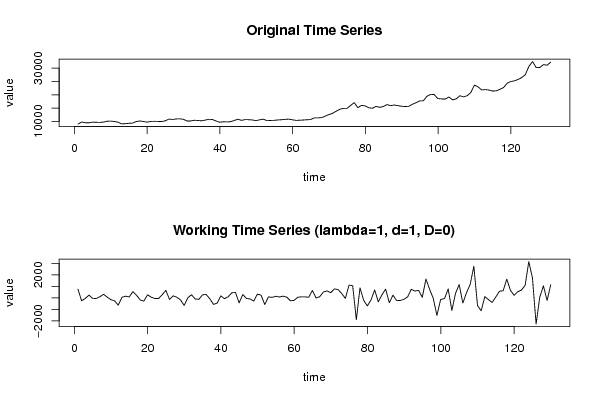
Dataseries X:

Download CSV

Histogram

Boxplots

Summary of computational transaction
Raw Input	view raw input (R code)
Raw Output	view raw output of R engine
Computing time	2 seconds
R Server	'Gwilym Jenkins' @ 72.249.127.135

\begin{tabular}{lllllllll}
\hline
Summary of computational transaction \tabularnewline
Raw Input & view raw input (R code)  \tabularnewline
Raw Output & view raw output of R engine  \tabularnewline
Computing time & 2 seconds \tabularnewline
R Server & 'Gwilym Jenkins' @ 72.249.127.135 \tabularnewline
\hline
\end{tabular}
%Source: https://freestatistics.org/blog/index.php?pk=112868&T=0

[TABLE]
[ROW][C]Summary of computational transaction[/C][/ROW]
[ROW][C]Raw Input[/C][C]view raw input (R code) [/C][/ROW]
[ROW][C]Raw Output[/C][C]view raw output of R engine [/C][/ROW]
[ROW][C]Computing time[/C][C]2 seconds[/C][/ROW]
[ROW][C]R Server[/C][C]'Gwilym Jenkins' @ 72.249.127.135[/C][/ROW]
[/TABLE]
Source: https://freestatistics.org/blog/index.php?pk=112868&T=0

Globally Unique Identifier (entire table): ba.freestatistics.org/blog/index.php?pk=112868&T=0

As an alternative you can also use a QR Code:

The GUIDs for individual cells are displayed in the table below:

Summary of computational transaction
Raw Input	view raw input (R code)
Raw Output	view raw output of R engine
Computing time	2 seconds
R Server	'Gwilym Jenkins' @ 72.249.127.135

Autocorrelation Function
Time lag k	ACF(k)	T-STAT	P-value
1	0.117449	1.3391	0.091433
2	-0.161636	-1.8429	0.033808
3	0.080328	0.9159	0.180714
4	0.074291	0.847	0.199264
5	-0.079816	-0.91	0.182242
6	0.006419	0.0732	0.470883
7	0.084176	0.9598	0.16948
8	-0.043173	-0.4922	0.311687
9	0.041252	0.4703	0.319448
10	-0.062054	-0.7075	0.240252
11	0.065097	0.7422	0.229647
12	0.107108	1.2212	0.112107
13	0.032456	0.3701	0.355973
14	-0.051004	-0.5815	0.280942
15	0.151989	1.7329	0.042739
16	0.139775	1.5937	0.056718
17	-0.119604	-1.3637	0.087509
18	-0.084392	-0.9622	0.168863
19	-0.040726	-0.4644	0.321586
20	0.058761	0.67	0.252028
21	-0.015776	-0.1799	0.428764
22	0.09401	1.0719	0.142881
23	0.079427	0.9056	0.183411
24	-0.027966	-0.3189	0.375171
25	-0.043464	-0.4956	0.31052
26	0.061687	0.7033	0.241551
27	0.115909	1.3216	0.094317
28	0.047802	0.545	0.293336
29	-0.011877	-0.1354	0.446245
30	-0.051569	-0.588	0.278785
31	0.023719	0.2704	0.393628
32	-0.032337	-0.3687	0.356475
33	0.040372	0.4603	0.323031
34	0.047841	0.5455	0.293182
35	-0.076884	-0.8766	0.191157
36	0.006848	0.0781	0.468942
37	0.019103	0.2178	0.413961
38	-0.022181	-0.2529	0.400371
39	0.001151	0.0131	0.494775
40	0.065135	0.7427	0.229515
41	-0.079427	-0.9056	0.183411
42	-0.038193	-0.4355	0.331972
43	0.04777	0.5447	0.29346
44	-0.087836	-1.0015	0.159227
45	-0.05607	-0.6393	0.261879
46	0.056061	0.6392	0.261911
47	0.001168	0.0133	0.494697
48	-0.019846	-0.2263	0.410668
49	0.147655	1.6835	0.047337
50	0.030956	0.3529	0.36235
51	-0.012041	-0.1373	0.445508
52	0.085544	0.9753	0.1656
53	0.01249	0.1424	0.44349
54	0.050157	0.5719	0.284197
55	-0.002407	-0.0274	0.489072
56	-0.018765	-0.214	0.415458
57	-0.065915	-0.7516	0.22684
58	-0.002825	-0.0322	0.487177
59	0.018354	0.2093	0.417285
60	-0.012421	-0.1416	0.443797

\begin{tabular}{lllllllll}
\hline
Autocorrelation Function \tabularnewline
Time lag k & ACF(k) & T-STAT & P-value \tabularnewline
1 & 0.117449 & 1.3391 & 0.091433 \tabularnewline
2 & -0.161636 & -1.8429 & 0.033808 \tabularnewline
3 & 0.080328 & 0.9159 & 0.180714 \tabularnewline
4 & 0.074291 & 0.847 & 0.199264 \tabularnewline
5 & -0.079816 & -0.91 & 0.182242 \tabularnewline
6 & 0.006419 & 0.0732 & 0.470883 \tabularnewline
7 & 0.084176 & 0.9598 & 0.16948 \tabularnewline
8 & -0.043173 & -0.4922 & 0.311687 \tabularnewline
9 & 0.041252 & 0.4703 & 0.319448 \tabularnewline
10 & -0.062054 & -0.7075 & 0.240252 \tabularnewline
11 & 0.065097 & 0.7422 & 0.229647 \tabularnewline
12 & 0.107108 & 1.2212 & 0.112107 \tabularnewline
13 & 0.032456 & 0.3701 & 0.355973 \tabularnewline
14 & -0.051004 & -0.5815 & 0.280942 \tabularnewline
15 & 0.151989 & 1.7329 & 0.042739 \tabularnewline
16 & 0.139775 & 1.5937 & 0.056718 \tabularnewline
17 & -0.119604 & -1.3637 & 0.087509 \tabularnewline
18 & -0.084392 & -0.9622 & 0.168863 \tabularnewline
19 & -0.040726 & -0.4644 & 0.321586 \tabularnewline
20 & 0.058761 & 0.67 & 0.252028 \tabularnewline
21 & -0.015776 & -0.1799 & 0.428764 \tabularnewline
22 & 0.09401 & 1.0719 & 0.142881 \tabularnewline
23 & 0.079427 & 0.9056 & 0.183411 \tabularnewline
24 & -0.027966 & -0.3189 & 0.375171 \tabularnewline
25 & -0.043464 & -0.4956 & 0.31052 \tabularnewline
26 & 0.061687 & 0.7033 & 0.241551 \tabularnewline
27 & 0.115909 & 1.3216 & 0.094317 \tabularnewline
28 & 0.047802 & 0.545 & 0.293336 \tabularnewline
29 & -0.011877 & -0.1354 & 0.446245 \tabularnewline
30 & -0.051569 & -0.588 & 0.278785 \tabularnewline
31 & 0.023719 & 0.2704 & 0.393628 \tabularnewline
32 & -0.032337 & -0.3687 & 0.356475 \tabularnewline
33 & 0.040372 & 0.4603 & 0.323031 \tabularnewline
34 & 0.047841 & 0.5455 & 0.293182 \tabularnewline
35 & -0.076884 & -0.8766 & 0.191157 \tabularnewline
36 & 0.006848 & 0.0781 & 0.468942 \tabularnewline
37 & 0.019103 & 0.2178 & 0.413961 \tabularnewline
38 & -0.022181 & -0.2529 & 0.400371 \tabularnewline
39 & 0.001151 & 0.0131 & 0.494775 \tabularnewline
40 & 0.065135 & 0.7427 & 0.229515 \tabularnewline
41 & -0.079427 & -0.9056 & 0.183411 \tabularnewline
42 & -0.038193 & -0.4355 & 0.331972 \tabularnewline
43 & 0.04777 & 0.5447 & 0.29346 \tabularnewline
44 & -0.087836 & -1.0015 & 0.159227 \tabularnewline
45 & -0.05607 & -0.6393 & 0.261879 \tabularnewline
46 & 0.056061 & 0.6392 & 0.261911 \tabularnewline
47 & 0.001168 & 0.0133 & 0.494697 \tabularnewline
48 & -0.019846 & -0.2263 & 0.410668 \tabularnewline
49 & 0.147655 & 1.6835 & 0.047337 \tabularnewline
50 & 0.030956 & 0.3529 & 0.36235 \tabularnewline
51 & -0.012041 & -0.1373 & 0.445508 \tabularnewline
52 & 0.085544 & 0.9753 & 0.1656 \tabularnewline
53 & 0.01249 & 0.1424 & 0.44349 \tabularnewline
54 & 0.050157 & 0.5719 & 0.284197 \tabularnewline
55 & -0.002407 & -0.0274 & 0.489072 \tabularnewline
56 & -0.018765 & -0.214 & 0.415458 \tabularnewline
57 & -0.065915 & -0.7516 & 0.22684 \tabularnewline
58 & -0.002825 & -0.0322 & 0.487177 \tabularnewline
59 & 0.018354 & 0.2093 & 0.417285 \tabularnewline
60 & -0.012421 & -0.1416 & 0.443797 \tabularnewline
\hline
\end{tabular}
%Source: https://freestatistics.org/blog/index.php?pk=112868&T=1

[TABLE]
[ROW][C]Autocorrelation Function[/C][/ROW]
[ROW][C]Time lag k[/C][C]ACF(k)[/C][C]T-STAT[/C][C]P-value[/C][/ROW]
[ROW][C]1[/C][C]0.117449[/C][C]1.3391[/C][C]0.091433[/C][/ROW]
[ROW][C]2[/C][C]-0.161636[/C][C]-1.8429[/C][C]0.033808[/C][/ROW]
[ROW][C]3[/C][C]0.080328[/C][C]0.9159[/C][C]0.180714[/C][/ROW]
[ROW][C]4[/C][C]0.074291[/C][C]0.847[/C][C]0.199264[/C][/ROW]
[ROW][C]5[/C][C]-0.079816[/C][C]-0.91[/C][C]0.182242[/C][/ROW]
[ROW][C]6[/C][C]0.006419[/C][C]0.0732[/C][C]0.470883[/C][/ROW]
[ROW][C]7[/C][C]0.084176[/C][C]0.9598[/C][C]0.16948[/C][/ROW]
[ROW][C]8[/C][C]-0.043173[/C][C]-0.4922[/C][C]0.311687[/C][/ROW]
[ROW][C]9[/C][C]0.041252[/C][C]0.4703[/C][C]0.319448[/C][/ROW]
[ROW][C]10[/C][C]-0.062054[/C][C]-0.7075[/C][C]0.240252[/C][/ROW]
[ROW][C]11[/C][C]0.065097[/C][C]0.7422[/C][C]0.229647[/C][/ROW]
[ROW][C]12[/C][C]0.107108[/C][C]1.2212[/C][C]0.112107[/C][/ROW]
[ROW][C]13[/C][C]0.032456[/C][C]0.3701[/C][C]0.355973[/C][/ROW]
[ROW][C]14[/C][C]-0.051004[/C][C]-0.5815[/C][C]0.280942[/C][/ROW]
[ROW][C]15[/C][C]0.151989[/C][C]1.7329[/C][C]0.042739[/C][/ROW]
[ROW][C]16[/C][C]0.139775[/C][C]1.5937[/C][C]0.056718[/C][/ROW]
[ROW][C]17[/C][C]-0.119604[/C][C]-1.3637[/C][C]0.087509[/C][/ROW]
[ROW][C]18[/C][C]-0.084392[/C][C]-0.9622[/C][C]0.168863[/C][/ROW]
[ROW][C]19[/C][C]-0.040726[/C][C]-0.4644[/C][C]0.321586[/C][/ROW]
[ROW][C]20[/C][C]0.058761[/C][C]0.67[/C][C]0.252028[/C][/ROW]
[ROW][C]21[/C][C]-0.015776[/C][C]-0.1799[/C][C]0.428764[/C][/ROW]
[ROW][C]22[/C][C]0.09401[/C][C]1.0719[/C][C]0.142881[/C][/ROW]
[ROW][C]23[/C][C]0.079427[/C][C]0.9056[/C][C]0.183411[/C][/ROW]
[ROW][C]24[/C][C]-0.027966[/C][C]-0.3189[/C][C]0.375171[/C][/ROW]
[ROW][C]25[/C][C]-0.043464[/C][C]-0.4956[/C][C]0.31052[/C][/ROW]
[ROW][C]26[/C][C]0.061687[/C][C]0.7033[/C][C]0.241551[/C][/ROW]
[ROW][C]27[/C][C]0.115909[/C][C]1.3216[/C][C]0.094317[/C][/ROW]
[ROW][C]28[/C][C]0.047802[/C][C]0.545[/C][C]0.293336[/C][/ROW]
[ROW][C]29[/C][C]-0.011877[/C][C]-0.1354[/C][C]0.446245[/C][/ROW]
[ROW][C]30[/C][C]-0.051569[/C][C]-0.588[/C][C]0.278785[/C][/ROW]
[ROW][C]31[/C][C]0.023719[/C][C]0.2704[/C][C]0.393628[/C][/ROW]
[ROW][C]32[/C][C]-0.032337[/C][C]-0.3687[/C][C]0.356475[/C][/ROW]
[ROW][C]33[/C][C]0.040372[/C][C]0.4603[/C][C]0.323031[/C][/ROW]
[ROW][C]34[/C][C]0.047841[/C][C]0.5455[/C][C]0.293182[/C][/ROW]
[ROW][C]35[/C][C]-0.076884[/C][C]-0.8766[/C][C]0.191157[/C][/ROW]
[ROW][C]36[/C][C]0.006848[/C][C]0.0781[/C][C]0.468942[/C][/ROW]
[ROW][C]37[/C][C]0.019103[/C][C]0.2178[/C][C]0.413961[/C][/ROW]
[ROW][C]38[/C][C]-0.022181[/C][C]-0.2529[/C][C]0.400371[/C][/ROW]
[ROW][C]39[/C][C]0.001151[/C][C]0.0131[/C][C]0.494775[/C][/ROW]
[ROW][C]40[/C][C]0.065135[/C][C]0.7427[/C][C]0.229515[/C][/ROW]
[ROW][C]41[/C][C]-0.079427[/C][C]-0.9056[/C][C]0.183411[/C][/ROW]
[ROW][C]42[/C][C]-0.038193[/C][C]-0.4355[/C][C]0.331972[/C][/ROW]
[ROW][C]43[/C][C]0.04777[/C][C]0.5447[/C][C]0.29346[/C][/ROW]
[ROW][C]44[/C][C]-0.087836[/C][C]-1.0015[/C][C]0.159227[/C][/ROW]
[ROW][C]45[/C][C]-0.05607[/C][C]-0.6393[/C][C]0.261879[/C][/ROW]
[ROW][C]46[/C][C]0.056061[/C][C]0.6392[/C][C]0.261911[/C][/ROW]
[ROW][C]47[/C][C]0.001168[/C][C]0.0133[/C][C]0.494697[/C][/ROW]
[ROW][C]48[/C][C]-0.019846[/C][C]-0.2263[/C][C]0.410668[/C][/ROW]
[ROW][C]49[/C][C]0.147655[/C][C]1.6835[/C][C]0.047337[/C][/ROW]
[ROW][C]50[/C][C]0.030956[/C][C]0.3529[/C][C]0.36235[/C][/ROW]
[ROW][C]51[/C][C]-0.012041[/C][C]-0.1373[/C][C]0.445508[/C][/ROW]
[ROW][C]52[/C][C]0.085544[/C][C]0.9753[/C][C]0.1656[/C][/ROW]
[ROW][C]53[/C][C]0.01249[/C][C]0.1424[/C][C]0.44349[/C][/ROW]
[ROW][C]54[/C][C]0.050157[/C][C]0.5719[/C][C]0.284197[/C][/ROW]
[ROW][C]55[/C][C]-0.002407[/C][C]-0.0274[/C][C]0.489072[/C][/ROW]
[ROW][C]56[/C][C]-0.018765[/C][C]-0.214[/C][C]0.415458[/C][/ROW]
[ROW][C]57[/C][C]-0.065915[/C][C]-0.7516[/C][C]0.22684[/C][/ROW]
[ROW][C]58[/C][C]-0.002825[/C][C]-0.0322[/C][C]0.487177[/C][/ROW]
[ROW][C]59[/C][C]0.018354[/C][C]0.2093[/C][C]0.417285[/C][/ROW]
[ROW][C]60[/C][C]-0.012421[/C][C]-0.1416[/C][C]0.443797[/C][/ROW]
[/TABLE]
Source: https://freestatistics.org/blog/index.php?pk=112868&T=1

Globally Unique Identifier (entire table): ba.freestatistics.org/blog/index.php?pk=112868&T=1

As an alternative you can also use a QR Code:

The GUIDs for individual cells are displayed in the table below:

Autocorrelation Function
Time lag k	ACF(k)	T-STAT	P-value
1	0.117449	1.3391	0.091433
2	-0.161636	-1.8429	0.033808
3	0.080328	0.9159	0.180714
4	0.074291	0.847	0.199264
5	-0.079816	-0.91	0.182242
6	0.006419	0.0732	0.470883
7	0.084176	0.9598	0.16948
8	-0.043173	-0.4922	0.311687
9	0.041252	0.4703	0.319448
10	-0.062054	-0.7075	0.240252
11	0.065097	0.7422	0.229647
12	0.107108	1.2212	0.112107
13	0.032456	0.3701	0.355973
14	-0.051004	-0.5815	0.280942
15	0.151989	1.7329	0.042739
16	0.139775	1.5937	0.056718
17	-0.119604	-1.3637	0.087509
18	-0.084392	-0.9622	0.168863
19	-0.040726	-0.4644	0.321586
20	0.058761	0.67	0.252028
21	-0.015776	-0.1799	0.428764
22	0.09401	1.0719	0.142881
23	0.079427	0.9056	0.183411
24	-0.027966	-0.3189	0.375171
25	-0.043464	-0.4956	0.31052
26	0.061687	0.7033	0.241551
27	0.115909	1.3216	0.094317
28	0.047802	0.545	0.293336
29	-0.011877	-0.1354	0.446245
30	-0.051569	-0.588	0.278785
31	0.023719	0.2704	0.393628
32	-0.032337	-0.3687	0.356475
33	0.040372	0.4603	0.323031
34	0.047841	0.5455	0.293182
35	-0.076884	-0.8766	0.191157
36	0.006848	0.0781	0.468942
37	0.019103	0.2178	0.413961
38	-0.022181	-0.2529	0.400371
39	0.001151	0.0131	0.494775
40	0.065135	0.7427	0.229515
41	-0.079427	-0.9056	0.183411
42	-0.038193	-0.4355	0.331972
43	0.04777	0.5447	0.29346
44	-0.087836	-1.0015	0.159227
45	-0.05607	-0.6393	0.261879
46	0.056061	0.6392	0.261911
47	0.001168	0.0133	0.494697
48	-0.019846	-0.2263	0.410668
49	0.147655	1.6835	0.047337
50	0.030956	0.3529	0.36235
51	-0.012041	-0.1373	0.445508
52	0.085544	0.9753	0.1656
53	0.01249	0.1424	0.44349
54	0.050157	0.5719	0.284197
55	-0.002407	-0.0274	0.489072
56	-0.018765	-0.214	0.415458
57	-0.065915	-0.7516	0.22684
58	-0.002825	-0.0322	0.487177
59	0.018354	0.2093	0.417285
60	-0.012421	-0.1416	0.443797

Partial Autocorrelation Function
Time lag k	PACF(k)	T-STAT	P-value
1	0.117449	1.3391	0.091433
2	-0.177884	-2.0282	0.022292
3	0.129404	1.4754	0.071257
4	0.015425	0.1759	0.430334
5	-0.061216	-0.698	0.243222
6	0.037391	0.4263	0.335287
7	0.045212	0.5155	0.303542
8	-0.047807	-0.5451	0.293316
9	0.087733	1.0003	0.15951
10	-0.127062	-1.4487	0.074911
11	0.133475	1.5218	0.065238
12	0.050965	0.5811	0.281092
13	0.037714	0.43	0.333952
14	-0.03497	-0.3987	0.345375
15	0.165328	1.885	0.030829
16	0.06122	0.698	0.243206
17	-0.069511	-0.7925	0.214744
18	-0.077867	-0.8878	0.188139
19	-0.084788	-0.9667	0.167738
20	0.078027	0.8896	0.18765
21	-0.013189	-0.1504	0.440349
22	0.107765	1.2287	0.1107
23	0.037966	0.4329	0.332908
24	-0.039742	-0.4531	0.325605
25	-0.012428	-0.1417	0.443769
26	0.059195	0.6749	0.250462
27	0.041099	0.4686	0.32007
28	0.065681	0.7489	0.227643
29	-0.03435	-0.3917	0.347978
30	-0.020474	-0.2334	0.407892
31	-0.014547	-0.1659	0.434261
32	-0.02751	-0.3137	0.377139
33	0.097574	1.1125	0.133985
34	0.025527	0.2911	0.385735
35	-0.128139	-1.461	0.073213
36	0.040675	0.4638	0.321796
37	-0.057394	-0.6544	0.257009
38	-0.046402	-0.5291	0.298831
39	0.044158	0.5035	0.307738
40	0.040869	0.466	0.321003
41	-0.069803	-0.7959	0.213777
42	-0.032646	-0.3722	0.355165
43	-0.031772	-0.3623	0.358873
44	-0.082115	-0.9363	0.175438
45	0.018739	0.2137	0.415577
46	0.046646	0.5318	0.297869
47	0.007195	0.082	0.467373
48	-0.003394	-0.0387	0.484594
49	0.074099	0.8449	0.199871
50	0.030888	0.3522	0.362638
51	0.067474	0.7693	0.221549
52	0.076667	0.8741	0.191828
53	-0.007455	-0.085	0.466196
54	0.077932	0.8886	0.187941
55	-0.086099	-0.9817	0.164041
56	-0.003593	-0.041	0.483692
57	-0.00299	-0.0341	0.486428
58	0.003209	0.0366	0.485433
59	0.031334	0.3573	0.360739
60	-0.031533	-0.3595	0.35989

\begin{tabular}{lllllllll}
\hline
Partial Autocorrelation Function \tabularnewline
Time lag k & PACF(k) & T-STAT & P-value \tabularnewline
1 & 0.117449 & 1.3391 & 0.091433 \tabularnewline
2 & -0.177884 & -2.0282 & 0.022292 \tabularnewline
3 & 0.129404 & 1.4754 & 0.071257 \tabularnewline
4 & 0.015425 & 0.1759 & 0.430334 \tabularnewline
5 & -0.061216 & -0.698 & 0.243222 \tabularnewline
6 & 0.037391 & 0.4263 & 0.335287 \tabularnewline
7 & 0.045212 & 0.5155 & 0.303542 \tabularnewline
8 & -0.047807 & -0.5451 & 0.293316 \tabularnewline
9 & 0.087733 & 1.0003 & 0.15951 \tabularnewline
10 & -0.127062 & -1.4487 & 0.074911 \tabularnewline
11 & 0.133475 & 1.5218 & 0.065238 \tabularnewline
12 & 0.050965 & 0.5811 & 0.281092 \tabularnewline
13 & 0.037714 & 0.43 & 0.333952 \tabularnewline
14 & -0.03497 & -0.3987 & 0.345375 \tabularnewline
15 & 0.165328 & 1.885 & 0.030829 \tabularnewline
16 & 0.06122 & 0.698 & 0.243206 \tabularnewline
17 & -0.069511 & -0.7925 & 0.214744 \tabularnewline
18 & -0.077867 & -0.8878 & 0.188139 \tabularnewline
19 & -0.084788 & -0.9667 & 0.167738 \tabularnewline
20 & 0.078027 & 0.8896 & 0.18765 \tabularnewline
21 & -0.013189 & -0.1504 & 0.440349 \tabularnewline
22 & 0.107765 & 1.2287 & 0.1107 \tabularnewline
23 & 0.037966 & 0.4329 & 0.332908 \tabularnewline
24 & -0.039742 & -0.4531 & 0.325605 \tabularnewline
25 & -0.012428 & -0.1417 & 0.443769 \tabularnewline
26 & 0.059195 & 0.6749 & 0.250462 \tabularnewline
27 & 0.041099 & 0.4686 & 0.32007 \tabularnewline
28 & 0.065681 & 0.7489 & 0.227643 \tabularnewline
29 & -0.03435 & -0.3917 & 0.347978 \tabularnewline
30 & -0.020474 & -0.2334 & 0.407892 \tabularnewline
31 & -0.014547 & -0.1659 & 0.434261 \tabularnewline
32 & -0.02751 & -0.3137 & 0.377139 \tabularnewline
33 & 0.097574 & 1.1125 & 0.133985 \tabularnewline
34 & 0.025527 & 0.2911 & 0.385735 \tabularnewline
35 & -0.128139 & -1.461 & 0.073213 \tabularnewline
36 & 0.040675 & 0.4638 & 0.321796 \tabularnewline
37 & -0.057394 & -0.6544 & 0.257009 \tabularnewline
38 & -0.046402 & -0.5291 & 0.298831 \tabularnewline
39 & 0.044158 & 0.5035 & 0.307738 \tabularnewline
40 & 0.040869 & 0.466 & 0.321003 \tabularnewline
41 & -0.069803 & -0.7959 & 0.213777 \tabularnewline
42 & -0.032646 & -0.3722 & 0.355165 \tabularnewline
43 & -0.031772 & -0.3623 & 0.358873 \tabularnewline
44 & -0.082115 & -0.9363 & 0.175438 \tabularnewline
45 & 0.018739 & 0.2137 & 0.415577 \tabularnewline
46 & 0.046646 & 0.5318 & 0.297869 \tabularnewline
47 & 0.007195 & 0.082 & 0.467373 \tabularnewline
48 & -0.003394 & -0.0387 & 0.484594 \tabularnewline
49 & 0.074099 & 0.8449 & 0.199871 \tabularnewline
50 & 0.030888 & 0.3522 & 0.362638 \tabularnewline
51 & 0.067474 & 0.7693 & 0.221549 \tabularnewline
52 & 0.076667 & 0.8741 & 0.191828 \tabularnewline
53 & -0.007455 & -0.085 & 0.466196 \tabularnewline
54 & 0.077932 & 0.8886 & 0.187941 \tabularnewline
55 & -0.086099 & -0.9817 & 0.164041 \tabularnewline
56 & -0.003593 & -0.041 & 0.483692 \tabularnewline
57 & -0.00299 & -0.0341 & 0.486428 \tabularnewline
58 & 0.003209 & 0.0366 & 0.485433 \tabularnewline
59 & 0.031334 & 0.3573 & 0.360739 \tabularnewline
60 & -0.031533 & -0.3595 & 0.35989 \tabularnewline
\hline
\end{tabular}
%Source: https://freestatistics.org/blog/index.php?pk=112868&T=2

[TABLE]
[ROW][C]Partial Autocorrelation Function[/C][/ROW]
[ROW][C]Time lag k[/C][C]PACF(k)[/C][C]T-STAT[/C][C]P-value[/C][/ROW]
[ROW][C]1[/C][C]0.117449[/C][C]1.3391[/C][C]0.091433[/C][/ROW]
[ROW][C]2[/C][C]-0.177884[/C][C]-2.0282[/C][C]0.022292[/C][/ROW]
[ROW][C]3[/C][C]0.129404[/C][C]1.4754[/C][C]0.071257[/C][/ROW]
[ROW][C]4[/C][C]0.015425[/C][C]0.1759[/C][C]0.430334[/C][/ROW]
[ROW][C]5[/C][C]-0.061216[/C][C]-0.698[/C][C]0.243222[/C][/ROW]
[ROW][C]6[/C][C]0.037391[/C][C]0.4263[/C][C]0.335287[/C][/ROW]
[ROW][C]7[/C][C]0.045212[/C][C]0.5155[/C][C]0.303542[/C][/ROW]
[ROW][C]8[/C][C]-0.047807[/C][C]-0.5451[/C][C]0.293316[/C][/ROW]
[ROW][C]9[/C][C]0.087733[/C][C]1.0003[/C][C]0.15951[/C][/ROW]
[ROW][C]10[/C][C]-0.127062[/C][C]-1.4487[/C][C]0.074911[/C][/ROW]
[ROW][C]11[/C][C]0.133475[/C][C]1.5218[/C][C]0.065238[/C][/ROW]
[ROW][C]12[/C][C]0.050965[/C][C]0.5811[/C][C]0.281092[/C][/ROW]
[ROW][C]13[/C][C]0.037714[/C][C]0.43[/C][C]0.333952[/C][/ROW]
[ROW][C]14[/C][C]-0.03497[/C][C]-0.3987[/C][C]0.345375[/C][/ROW]
[ROW][C]15[/C][C]0.165328[/C][C]1.885[/C][C]0.030829[/C][/ROW]
[ROW][C]16[/C][C]0.06122[/C][C]0.698[/C][C]0.243206[/C][/ROW]
[ROW][C]17[/C][C]-0.069511[/C][C]-0.7925[/C][C]0.214744[/C][/ROW]
[ROW][C]18[/C][C]-0.077867[/C][C]-0.8878[/C][C]0.188139[/C][/ROW]
[ROW][C]19[/C][C]-0.084788[/C][C]-0.9667[/C][C]0.167738[/C][/ROW]
[ROW][C]20[/C][C]0.078027[/C][C]0.8896[/C][C]0.18765[/C][/ROW]
[ROW][C]21[/C][C]-0.013189[/C][C]-0.1504[/C][C]0.440349[/C][/ROW]
[ROW][C]22[/C][C]0.107765[/C][C]1.2287[/C][C]0.1107[/C][/ROW]
[ROW][C]23[/C][C]0.037966[/C][C]0.4329[/C][C]0.332908[/C][/ROW]
[ROW][C]24[/C][C]-0.039742[/C][C]-0.4531[/C][C]0.325605[/C][/ROW]
[ROW][C]25[/C][C]-0.012428[/C][C]-0.1417[/C][C]0.443769[/C][/ROW]
[ROW][C]26[/C][C]0.059195[/C][C]0.6749[/C][C]0.250462[/C][/ROW]
[ROW][C]27[/C][C]0.041099[/C][C]0.4686[/C][C]0.32007[/C][/ROW]
[ROW][C]28[/C][C]0.065681[/C][C]0.7489[/C][C]0.227643[/C][/ROW]
[ROW][C]29[/C][C]-0.03435[/C][C]-0.3917[/C][C]0.347978[/C][/ROW]
[ROW][C]30[/C][C]-0.020474[/C][C]-0.2334[/C][C]0.407892[/C][/ROW]
[ROW][C]31[/C][C]-0.014547[/C][C]-0.1659[/C][C]0.434261[/C][/ROW]
[ROW][C]32[/C][C]-0.02751[/C][C]-0.3137[/C][C]0.377139[/C][/ROW]
[ROW][C]33[/C][C]0.097574[/C][C]1.1125[/C][C]0.133985[/C][/ROW]
[ROW][C]34[/C][C]0.025527[/C][C]0.2911[/C][C]0.385735[/C][/ROW]
[ROW][C]35[/C][C]-0.128139[/C][C]-1.461[/C][C]0.073213[/C][/ROW]
[ROW][C]36[/C][C]0.040675[/C][C]0.4638[/C][C]0.321796[/C][/ROW]
[ROW][C]37[/C][C]-0.057394[/C][C]-0.6544[/C][C]0.257009[/C][/ROW]
[ROW][C]38[/C][C]-0.046402[/C][C]-0.5291[/C][C]0.298831[/C][/ROW]
[ROW][C]39[/C][C]0.044158[/C][C]0.5035[/C][C]0.307738[/C][/ROW]
[ROW][C]40[/C][C]0.040869[/C][C]0.466[/C][C]0.321003[/C][/ROW]
[ROW][C]41[/C][C]-0.069803[/C][C]-0.7959[/C][C]0.213777[/C][/ROW]
[ROW][C]42[/C][C]-0.032646[/C][C]-0.3722[/C][C]0.355165[/C][/ROW]
[ROW][C]43[/C][C]-0.031772[/C][C]-0.3623[/C][C]0.358873[/C][/ROW]
[ROW][C]44[/C][C]-0.082115[/C][C]-0.9363[/C][C]0.175438[/C][/ROW]
[ROW][C]45[/C][C]0.018739[/C][C]0.2137[/C][C]0.415577[/C][/ROW]
[ROW][C]46[/C][C]0.046646[/C][C]0.5318[/C][C]0.297869[/C][/ROW]
[ROW][C]47[/C][C]0.007195[/C][C]0.082[/C][C]0.467373[/C][/ROW]
[ROW][C]48[/C][C]-0.003394[/C][C]-0.0387[/C][C]0.484594[/C][/ROW]
[ROW][C]49[/C][C]0.074099[/C][C]0.8449[/C][C]0.199871[/C][/ROW]
[ROW][C]50[/C][C]0.030888[/C][C]0.3522[/C][C]0.362638[/C][/ROW]
[ROW][C]51[/C][C]0.067474[/C][C]0.7693[/C][C]0.221549[/C][/ROW]
[ROW][C]52[/C][C]0.076667[/C][C]0.8741[/C][C]0.191828[/C][/ROW]
[ROW][C]53[/C][C]-0.007455[/C][C]-0.085[/C][C]0.466196[/C][/ROW]
[ROW][C]54[/C][C]0.077932[/C][C]0.8886[/C][C]0.187941[/C][/ROW]
[ROW][C]55[/C][C]-0.086099[/C][C]-0.9817[/C][C]0.164041[/C][/ROW]
[ROW][C]56[/C][C]-0.003593[/C][C]-0.041[/C][C]0.483692[/C][/ROW]
[ROW][C]57[/C][C]-0.00299[/C][C]-0.0341[/C][C]0.486428[/C][/ROW]
[ROW][C]58[/C][C]0.003209[/C][C]0.0366[/C][C]0.485433[/C][/ROW]
[ROW][C]59[/C][C]0.031334[/C][C]0.3573[/C][C]0.360739[/C][/ROW]
[ROW][C]60[/C][C]-0.031533[/C][C]-0.3595[/C][C]0.35989[/C][/ROW]
[/TABLE]
Source: https://freestatistics.org/blog/index.php?pk=112868&T=2

Globally Unique Identifier (entire table): ba.freestatistics.org/blog/index.php?pk=112868&T=2

As an alternative you can also use a QR Code:

The GUIDs for individual cells are displayed in the table below:

Partial Autocorrelation Function
Time lag k	PACF(k)	T-STAT	P-value
1	0.117449	1.3391	0.091433
2	-0.177884	-2.0282	0.022292
3	0.129404	1.4754	0.071257
4	0.015425	0.1759	0.430334
5	-0.061216	-0.698	0.243222
6	0.037391	0.4263	0.335287
7	0.045212	0.5155	0.303542
8	-0.047807	-0.5451	0.293316
9	0.087733	1.0003	0.15951
10	-0.127062	-1.4487	0.074911
11	0.133475	1.5218	0.065238
12	0.050965	0.5811	0.281092
13	0.037714	0.43	0.333952
14	-0.03497	-0.3987	0.345375
15	0.165328	1.885	0.030829
16	0.06122	0.698	0.243206
17	-0.069511	-0.7925	0.214744
18	-0.077867	-0.8878	0.188139
19	-0.084788	-0.9667	0.167738
20	0.078027	0.8896	0.18765
21	-0.013189	-0.1504	0.440349
22	0.107765	1.2287	0.1107
23	0.037966	0.4329	0.332908
24	-0.039742	-0.4531	0.325605
25	-0.012428	-0.1417	0.443769
26	0.059195	0.6749	0.250462
27	0.041099	0.4686	0.32007
28	0.065681	0.7489	0.227643
29	-0.03435	-0.3917	0.347978
30	-0.020474	-0.2334	0.407892
31	-0.014547	-0.1659	0.434261
32	-0.02751	-0.3137	0.377139
33	0.097574	1.1125	0.133985
34	0.025527	0.2911	0.385735
35	-0.128139	-1.461	0.073213
36	0.040675	0.4638	0.321796
37	-0.057394	-0.6544	0.257009
38	-0.046402	-0.5291	0.298831
39	0.044158	0.5035	0.307738
40	0.040869	0.466	0.321003
41	-0.069803	-0.7959	0.213777
42	-0.032646	-0.3722	0.355165
43	-0.031772	-0.3623	0.358873
44	-0.082115	-0.9363	0.175438
45	0.018739	0.2137	0.415577
46	0.046646	0.5318	0.297869
47	0.007195	0.082	0.467373
48	-0.003394	-0.0387	0.484594
49	0.074099	0.8449	0.199871
50	0.030888	0.3522	0.362638
51	0.067474	0.7693	0.221549
52	0.076667	0.8741	0.191828
53	-0.007455	-0.085	0.466196
54	0.077932	0.8886	0.187941
55	-0.086099	-0.9817	0.164041
56	-0.003593	-0.041	0.483692
57	-0.00299	-0.0341	0.486428
58	0.003209	0.0366	0.485433
59	0.031334	0.3573	0.360739
60	-0.031533	-0.3595	0.35989

Figure 1

PNG link

Postscript link

PDF link

Figure 2

PNG link

Postscript link

PDF link

Figure 3

PNG link

Postscript link

PDF link

Parameters (Session):

par1 = 60 ; par2 = 1 ; par3 = 2 ; par4 = 0 ; par5 = 12 ; par6 = White Noise ; par7 = 0.95 ;

Parameters (R input):

par1 = 60 ; par2 = 1 ; par3 = 1 ; par4 = 0 ; par5 = 12 ; par6 = White Noise ; par7 = 0.95 ; par8 = ;

R code (references can be found in the software module):

if (par1 == 'Default') {
par1 = 10*log10(length(x))
} else {
par1 <- as.numeric(par1)
}
par2 <- as.numeric(par2)
par3 <- as.numeric(par3)
par4 <- as.numeric(par4)
par5 <- as.numeric(par5)
if (par6 == 'White Noise') par6 <- 'white' else par6 <- 'ma'
par7 <- as.numeric(par7)
if (par8 != '') par8 <- as.numeric(par8)
ox <- x
if (par8 == '') {
if (par2 == 0) {
x <- log(x)
} else {
x <- (x ^ par2 - 1) / par2
}
} else {
x <- log(x,base=par8)
}
if (par3 > 0) x <- diff(x,lag=1,difference=par3)
if (par4 > 0) x <- diff(x,lag=par5,difference=par4)
bitmap(file='picts.png')
op <- par(mfrow=c(2,1))
plot(ox,type='l',main='Original Time Series',xlab='time',ylab='value')
if (par8=='') {
mytitle <- paste('Working Time Series (lambda=',par2,', d=',par3,', D=',par4,')',sep='')
mysub <- paste('(lambda=',par2,', d=',par3,', D=',par4,', CI=', par7, ', CI type=',par6,')',sep='')
} else {
mytitle <- paste('Working Time Series (base=',par8,', d=',par3,', D=',par4,')',sep='')
mysub <- paste('(base=',par8,', d=',par3,', D=',par4,', CI=', par7, ', CI type=',par6,')',sep='')
}
plot(x,type='l', main=mytitle,xlab='time',ylab='value')
par(op)
dev.off()
bitmap(file='pic1.png')
racf <- acf(x, par1, main='Autocorrelation', xlab='time lag', ylab='ACF', ci.type=par6, ci=par7, sub=mysub)
dev.off()
bitmap(file='pic2.png')
rpacf <- pacf(x,par1,main='Partial Autocorrelation',xlab='lags',ylab='PACF',sub=mysub)
dev.off()
(myacf <- c(racf$acf))
(mypacf <- c(rpacf$acf))
lengthx <- length(x)
sqrtn <- sqrt(lengthx)
load(file='createtable')
a<-table.start()
a<-table.row.start(a)
a<-table.element(a,'Autocorrelation Function',4,TRUE)
a<-table.row.end(a)
a<-table.row.start(a)
a<-table.element(a,'Time lag k',header=TRUE)
a<-table.element(a,hyperlink('basics.htm','ACF(k)','click here for more information about the Autocorrelation Function'),header=TRUE)
a<-table.element(a,'T-STAT',header=TRUE)
a<-table.element(a,'P-value',header=TRUE)
a<-table.row.end(a)
for (i in 2:(par1+1)) {
a<-table.row.start(a)
a<-table.element(a,i-1,header=TRUE)
a<-table.element(a,round(myacf[i],6))
mytstat <- myacf[i]*sqrtn
a<-table.element(a,round(mytstat,4))
a<-table.element(a,round(1-pt(abs(mytstat),lengthx),6))
a<-table.row.end(a)
}
a<-table.end(a)
table.save(a,file='mytable.tab')
a<-table.start()
a<-table.row.start(a)
a<-table.element(a,'Partial Autocorrelation Function',4,TRUE)
a<-table.row.end(a)
a<-table.row.start(a)
a<-table.element(a,'Time lag k',header=TRUE)
a<-table.element(a,hyperlink('basics.htm','PACF(k)','click here for more information about the Partial Autocorrelation Function'),header=TRUE)
a<-table.element(a,'T-STAT',header=TRUE)
a<-table.element(a,'P-value',header=TRUE)
a<-table.row.end(a)
for (i in 1:par1) {
a<-table.row.start(a)
a<-table.element(a,i,header=TRUE)
a<-table.element(a,round(mypacf[i],6))
mytstat <- mypacf[i]*sqrtn
a<-table.element(a,round(mytstat,4))
a<-table.element(a,round(1-pt(abs(mytstat),lengthx),6))
a<-table.row.end(a)
}
a<-table.end(a)
table.save(a,file='mytable1.tab')

Free Statistics

Description of Statistical Computation

Tree of Dependent Computations

Dataset

Tables (Output of Computation)

Figures (Output of Computation)

Input Parameters & R Code