Free Statistics
of Irreproducible Research!
Description of Statistical Computation | |||||||||||||||||||||||||||||||||||||||||||||||||||||||||||||||||||||||||||||||||||||||||||||||||||||||||||||||||||||||||||||||||||||||||||||||||||||||||||||||||||||||||||||||||||||||||||||||||||||||||||||||||||||||||||||||||||||||||||||||||||||||||||||||||||||||||||||||||||||||||||||||||||||||||||||||||||||||||||||||||||||||||||||||||||||||||||||||||||||||||||||||||||||||||||||||||||||||||||||||||||||||||||||||||||||||||||||||||||||||||||||||||||||||||||||||||||||||||||||||||||||||||||||||||||||||||||||||||||||||||||||||||||||||||||||||||||||||||||||||||||||||||||||||||||||||||||||||||||||||||||||||||||||||||||||||||||||||||||||||||||||||||||||||||||||||||||||||||||||||||||||||||||||||||||||||
|---|---|---|---|---|---|---|---|---|---|---|---|---|---|---|---|---|---|---|---|---|---|---|---|---|---|---|---|---|---|---|---|---|---|---|---|---|---|---|---|---|---|---|---|---|---|---|---|---|---|---|---|---|---|---|---|---|---|---|---|---|---|---|---|---|---|---|---|---|---|---|---|---|---|---|---|---|---|---|---|---|---|---|---|---|---|---|---|---|---|---|---|---|---|---|---|---|---|---|---|---|---|---|---|---|---|---|---|---|---|---|---|---|---|---|---|---|---|---|---|---|---|---|---|---|---|---|---|---|---|---|---|---|---|---|---|---|---|---|---|---|---|---|---|---|---|---|---|---|---|---|---|---|---|---|---|---|---|---|---|---|---|---|---|---|---|---|---|---|---|---|---|---|---|---|---|---|---|---|---|---|---|---|---|---|---|---|---|---|---|---|---|---|---|---|---|---|---|---|---|---|---|---|---|---|---|---|---|---|---|---|---|---|---|---|---|---|---|---|---|---|---|---|---|---|---|---|---|---|---|---|---|---|---|---|---|---|---|---|---|---|---|---|---|---|---|---|---|---|---|---|---|---|---|---|---|---|---|---|---|---|---|---|---|---|---|---|---|---|---|---|---|---|---|---|---|---|---|---|---|---|---|---|---|---|---|---|---|---|---|---|---|---|---|---|---|---|---|---|---|---|---|---|---|---|---|---|---|---|---|---|---|---|---|---|---|---|---|---|---|---|---|---|---|---|---|---|---|---|---|---|---|---|---|---|---|---|---|---|---|---|---|---|---|---|---|---|---|---|---|---|---|---|---|---|---|---|---|---|---|---|---|---|---|---|---|---|---|---|---|---|---|---|---|---|---|---|---|---|---|---|---|---|---|---|---|---|---|---|---|---|---|---|---|---|---|---|---|---|---|---|---|---|---|---|---|---|---|---|---|---|---|---|---|---|---|---|---|---|---|---|---|---|---|---|---|---|---|---|---|---|---|---|---|---|---|---|---|---|---|---|---|---|---|---|---|---|---|---|---|---|---|---|---|---|---|---|---|---|---|---|---|---|---|---|---|---|---|---|---|---|---|---|---|---|---|---|---|---|---|---|---|---|---|---|---|---|---|---|---|---|---|---|---|---|---|---|---|---|---|---|---|---|---|---|---|---|---|---|---|---|---|---|---|---|---|---|---|---|---|---|---|---|---|---|---|---|---|---|---|---|---|---|---|---|---|---|---|---|---|---|---|---|---|---|---|---|---|---|---|---|---|---|---|---|---|---|---|---|---|---|---|---|---|---|---|---|---|---|---|---|---|---|---|---|---|---|---|---|---|---|---|---|---|---|---|---|---|---|---|---|---|---|---|---|---|---|---|---|---|---|---|---|---|---|---|---|---|---|---|---|---|---|---|---|---|---|---|---|---|---|---|---|---|---|---|---|---|---|---|---|---|---|---|---|---|---|---|---|---|---|---|---|---|---|---|---|---|---|---|---|---|---|---|---|---|---|---|---|---|---|---|---|---|---|---|---|---|---|---|---|---|---|---|---|---|---|---|---|---|---|---|---|---|---|---|---|---|---|---|---|---|---|---|---|---|---|---|---|---|---|---|---|---|
| Author's title | |||||||||||||||||||||||||||||||||||||||||||||||||||||||||||||||||||||||||||||||||||||||||||||||||||||||||||||||||||||||||||||||||||||||||||||||||||||||||||||||||||||||||||||||||||||||||||||||||||||||||||||||||||||||||||||||||||||||||||||||||||||||||||||||||||||||||||||||||||||||||||||||||||||||||||||||||||||||||||||||||||||||||||||||||||||||||||||||||||||||||||||||||||||||||||||||||||||||||||||||||||||||||||||||||||||||||||||||||||||||||||||||||||||||||||||||||||||||||||||||||||||||||||||||||||||||||||||||||||||||||||||||||||||||||||||||||||||||||||||||||||||||||||||||||||||||||||||||||||||||||||||||||||||||||||||||||||||||||||||||||||||||||||||||||||||||||||||||||||||||||||||||||||||||||||||||
| Author | *The author of this computation has been verified* | ||||||||||||||||||||||||||||||||||||||||||||||||||||||||||||||||||||||||||||||||||||||||||||||||||||||||||||||||||||||||||||||||||||||||||||||||||||||||||||||||||||||||||||||||||||||||||||||||||||||||||||||||||||||||||||||||||||||||||||||||||||||||||||||||||||||||||||||||||||||||||||||||||||||||||||||||||||||||||||||||||||||||||||||||||||||||||||||||||||||||||||||||||||||||||||||||||||||||||||||||||||||||||||||||||||||||||||||||||||||||||||||||||||||||||||||||||||||||||||||||||||||||||||||||||||||||||||||||||||||||||||||||||||||||||||||||||||||||||||||||||||||||||||||||||||||||||||||||||||||||||||||||||||||||||||||||||||||||||||||||||||||||||||||||||||||||||||||||||||||||||||||||||||||||||||||
| R Software Module | rwasp_arimaforecasting.wasp | ||||||||||||||||||||||||||||||||||||||||||||||||||||||||||||||||||||||||||||||||||||||||||||||||||||||||||||||||||||||||||||||||||||||||||||||||||||||||||||||||||||||||||||||||||||||||||||||||||||||||||||||||||||||||||||||||||||||||||||||||||||||||||||||||||||||||||||||||||||||||||||||||||||||||||||||||||||||||||||||||||||||||||||||||||||||||||||||||||||||||||||||||||||||||||||||||||||||||||||||||||||||||||||||||||||||||||||||||||||||||||||||||||||||||||||||||||||||||||||||||||||||||||||||||||||||||||||||||||||||||||||||||||||||||||||||||||||||||||||||||||||||||||||||||||||||||||||||||||||||||||||||||||||||||||||||||||||||||||||||||||||||||||||||||||||||||||||||||||||||||||||||||||||||||||||||
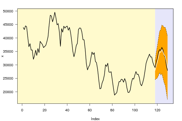
| Title produced by software | ARIMA Forecasting | ||||||||||||||||||||||||||||||||||||||||||||||||||||||||||||||||||||||||||||||||||||||||||||||||||||||||||||||||||||||||||||||||||||||||||||||||||||||||||||||||||||||||||||||||||||||||||||||||||||||||||||||||||||||||||||||||||||||||||||||||||||||||||||||||||||||||||||||||||||||||||||||||||||||||||||||||||||||||||||||||||||||||||||||||||||||||||||||||||||||||||||||||||||||||||||||||||||||||||||||||||||||||||||||||||||||||||||||||||||||||||||||||||||||||||||||||||||||||||||||||||||||||||||||||||||||||||||||||||||||||||||||||||||||||||||||||||||||||||||||||||||||||||||||||||||||||||||||||||||||||||||||||||||||||||||||||||||||||||||||||||||||||||||||||||||||||||||||||||||||||||||||||||||||||||||||
| Date of computation | Mon, 20 Dec 2010 10:13:32 +0000 | ||||||||||||||||||||||||||||||||||||||||||||||||||||||||||||||||||||||||||||||||||||||||||||||||||||||||||||||||||||||||||||||||||||||||||||||||||||||||||||||||||||||||||||||||||||||||||||||||||||||||||||||||||||||||||||||||||||||||||||||||||||||||||||||||||||||||||||||||||||||||||||||||||||||||||||||||||||||||||||||||||||||||||||||||||||||||||||||||||||||||||||||||||||||||||||||||||||||||||||||||||||||||||||||||||||||||||||||||||||||||||||||||||||||||||||||||||||||||||||||||||||||||||||||||||||||||||||||||||||||||||||||||||||||||||||||||||||||||||||||||||||||||||||||||||||||||||||||||||||||||||||||||||||||||||||||||||||||||||||||||||||||||||||||||||||||||||||||||||||||||||||||||||||||||||||||
| Cite this page as follows | Statistical Computations at FreeStatistics.org, Office for Research Development and Education, URL https://freestatistics.org/blog/index.php?v=date/2010/Dec/20/t12928398690jcpzqchu5604o2.htm/, Retrieved Sat, 04 May 2024 00:07:43 +0000 | ||||||||||||||||||||||||||||||||||||||||||||||||||||||||||||||||||||||||||||||||||||||||||||||||||||||||||||||||||||||||||||||||||||||||||||||||||||||||||||||||||||||||||||||||||||||||||||||||||||||||||||||||||||||||||||||||||||||||||||||||||||||||||||||||||||||||||||||||||||||||||||||||||||||||||||||||||||||||||||||||||||||||||||||||||||||||||||||||||||||||||||||||||||||||||||||||||||||||||||||||||||||||||||||||||||||||||||||||||||||||||||||||||||||||||||||||||||||||||||||||||||||||||||||||||||||||||||||||||||||||||||||||||||||||||||||||||||||||||||||||||||||||||||||||||||||||||||||||||||||||||||||||||||||||||||||||||||||||||||||||||||||||||||||||||||||||||||||||||||||||||||||||||||||||||||||
| Statistical Computations at FreeStatistics.org, Office for Research Development and Education, URL https://freestatistics.org/blog/index.php?pk=112824, Retrieved Sat, 04 May 2024 00:07:43 +0000 | |||||||||||||||||||||||||||||||||||||||||||||||||||||||||||||||||||||||||||||||||||||||||||||||||||||||||||||||||||||||||||||||||||||||||||||||||||||||||||||||||||||||||||||||||||||||||||||||||||||||||||||||||||||||||||||||||||||||||||||||||||||||||||||||||||||||||||||||||||||||||||||||||||||||||||||||||||||||||||||||||||||||||||||||||||||||||||||||||||||||||||||||||||||||||||||||||||||||||||||||||||||||||||||||||||||||||||||||||||||||||||||||||||||||||||||||||||||||||||||||||||||||||||||||||||||||||||||||||||||||||||||||||||||||||||||||||||||||||||||||||||||||||||||||||||||||||||||||||||||||||||||||||||||||||||||||||||||||||||||||||||||||||||||||||||||||||||||||||||||||||||||||||||||||||||||||
| QR Codes: | |||||||||||||||||||||||||||||||||||||||||||||||||||||||||||||||||||||||||||||||||||||||||||||||||||||||||||||||||||||||||||||||||||||||||||||||||||||||||||||||||||||||||||||||||||||||||||||||||||||||||||||||||||||||||||||||||||||||||||||||||||||||||||||||||||||||||||||||||||||||||||||||||||||||||||||||||||||||||||||||||||||||||||||||||||||||||||||||||||||||||||||||||||||||||||||||||||||||||||||||||||||||||||||||||||||||||||||||||||||||||||||||||||||||||||||||||||||||||||||||||||||||||||||||||||||||||||||||||||||||||||||||||||||||||||||||||||||||||||||||||||||||||||||||||||||||||||||||||||||||||||||||||||||||||||||||||||||||||||||||||||||||||||||||||||||||||||||||||||||||||||||||||||||||||||||||
|
| |||||||||||||||||||||||||||||||||||||||||||||||||||||||||||||||||||||||||||||||||||||||||||||||||||||||||||||||||||||||||||||||||||||||||||||||||||||||||||||||||||||||||||||||||||||||||||||||||||||||||||||||||||||||||||||||||||||||||||||||||||||||||||||||||||||||||||||||||||||||||||||||||||||||||||||||||||||||||||||||||||||||||||||||||||||||||||||||||||||||||||||||||||||||||||||||||||||||||||||||||||||||||||||||||||||||||||||||||||||||||||||||||||||||||||||||||||||||||||||||||||||||||||||||||||||||||||||||||||||||||||||||||||||||||||||||||||||||||||||||||||||||||||||||||||||||||||||||||||||||||||||||||||||||||||||||||||||||||||||||||||||||||||||||||||||||||||||||||||||||||||||||||||||||||||||||
| Original text written by user: | |||||||||||||||||||||||||||||||||||||||||||||||||||||||||||||||||||||||||||||||||||||||||||||||||||||||||||||||||||||||||||||||||||||||||||||||||||||||||||||||||||||||||||||||||||||||||||||||||||||||||||||||||||||||||||||||||||||||||||||||||||||||||||||||||||||||||||||||||||||||||||||||||||||||||||||||||||||||||||||||||||||||||||||||||||||||||||||||||||||||||||||||||||||||||||||||||||||||||||||||||||||||||||||||||||||||||||||||||||||||||||||||||||||||||||||||||||||||||||||||||||||||||||||||||||||||||||||||||||||||||||||||||||||||||||||||||||||||||||||||||||||||||||||||||||||||||||||||||||||||||||||||||||||||||||||||||||||||||||||||||||||||||||||||||||||||||||||||||||||||||||||||||||||||||||||||
| IsPrivate? | No (this computation is public) | ||||||||||||||||||||||||||||||||||||||||||||||||||||||||||||||||||||||||||||||||||||||||||||||||||||||||||||||||||||||||||||||||||||||||||||||||||||||||||||||||||||||||||||||||||||||||||||||||||||||||||||||||||||||||||||||||||||||||||||||||||||||||||||||||||||||||||||||||||||||||||||||||||||||||||||||||||||||||||||||||||||||||||||||||||||||||||||||||||||||||||||||||||||||||||||||||||||||||||||||||||||||||||||||||||||||||||||||||||||||||||||||||||||||||||||||||||||||||||||||||||||||||||||||||||||||||||||||||||||||||||||||||||||||||||||||||||||||||||||||||||||||||||||||||||||||||||||||||||||||||||||||||||||||||||||||||||||||||||||||||||||||||||||||||||||||||||||||||||||||||||||||||||||||||||||||
| User-defined keywords | |||||||||||||||||||||||||||||||||||||||||||||||||||||||||||||||||||||||||||||||||||||||||||||||||||||||||||||||||||||||||||||||||||||||||||||||||||||||||||||||||||||||||||||||||||||||||||||||||||||||||||||||||||||||||||||||||||||||||||||||||||||||||||||||||||||||||||||||||||||||||||||||||||||||||||||||||||||||||||||||||||||||||||||||||||||||||||||||||||||||||||||||||||||||||||||||||||||||||||||||||||||||||||||||||||||||||||||||||||||||||||||||||||||||||||||||||||||||||||||||||||||||||||||||||||||||||||||||||||||||||||||||||||||||||||||||||||||||||||||||||||||||||||||||||||||||||||||||||||||||||||||||||||||||||||||||||||||||||||||||||||||||||||||||||||||||||||||||||||||||||||||||||||||||||||||||
| Estimated Impact | 220 | ||||||||||||||||||||||||||||||||||||||||||||||||||||||||||||||||||||||||||||||||||||||||||||||||||||||||||||||||||||||||||||||||||||||||||||||||||||||||||||||||||||||||||||||||||||||||||||||||||||||||||||||||||||||||||||||||||||||||||||||||||||||||||||||||||||||||||||||||||||||||||||||||||||||||||||||||||||||||||||||||||||||||||||||||||||||||||||||||||||||||||||||||||||||||||||||||||||||||||||||||||||||||||||||||||||||||||||||||||||||||||||||||||||||||||||||||||||||||||||||||||||||||||||||||||||||||||||||||||||||||||||||||||||||||||||||||||||||||||||||||||||||||||||||||||||||||||||||||||||||||||||||||||||||||||||||||||||||||||||||||||||||||||||||||||||||||||||||||||||||||||||||||||||||||||||||
Tree of Dependent Computations | |||||||||||||||||||||||||||||||||||||||||||||||||||||||||||||||||||||||||||||||||||||||||||||||||||||||||||||||||||||||||||||||||||||||||||||||||||||||||||||||||||||||||||||||||||||||||||||||||||||||||||||||||||||||||||||||||||||||||||||||||||||||||||||||||||||||||||||||||||||||||||||||||||||||||||||||||||||||||||||||||||||||||||||||||||||||||||||||||||||||||||||||||||||||||||||||||||||||||||||||||||||||||||||||||||||||||||||||||||||||||||||||||||||||||||||||||||||||||||||||||||||||||||||||||||||||||||||||||||||||||||||||||||||||||||||||||||||||||||||||||||||||||||||||||||||||||||||||||||||||||||||||||||||||||||||||||||||||||||||||||||||||||||||||||||||||||||||||||||||||||||||||||||||||||||||||
| Family? (F = Feedback message, R = changed R code, M = changed R Module, P = changed Parameters, D = changed Data) | |||||||||||||||||||||||||||||||||||||||||||||||||||||||||||||||||||||||||||||||||||||||||||||||||||||||||||||||||||||||||||||||||||||||||||||||||||||||||||||||||||||||||||||||||||||||||||||||||||||||||||||||||||||||||||||||||||||||||||||||||||||||||||||||||||||||||||||||||||||||||||||||||||||||||||||||||||||||||||||||||||||||||||||||||||||||||||||||||||||||||||||||||||||||||||||||||||||||||||||||||||||||||||||||||||||||||||||||||||||||||||||||||||||||||||||||||||||||||||||||||||||||||||||||||||||||||||||||||||||||||||||||||||||||||||||||||||||||||||||||||||||||||||||||||||||||||||||||||||||||||||||||||||||||||||||||||||||||||||||||||||||||||||||||||||||||||||||||||||||||||||||||||||||||||||||||
| - [Univariate Data Series] [data set] [2008-12-01 19:54:57] [b98453cac15ba1066b407e146608df68] - RMP [Standard Deviation-Mean Plot] [Unemployment] [2010-11-29 10:34:47] [b98453cac15ba1066b407e146608df68] - RMP [ARIMA Backward Selection] [Unemployment] [2010-11-29 17:10:28] [b98453cac15ba1066b407e146608df68] - PD [ARIMA Backward Selection] [Arima - Parameter...] [2010-12-12 13:50:49] [aeb27d5c05332f2e597ad139ee63fbe4] - P [ARIMA Backward Selection] [Foutmelding Arima] [2010-12-17 08:18:10] [aeb27d5c05332f2e597ad139ee63fbe4] - RMP [ARIMA Forecasting] [] [2010-12-20 10:13:32] [d76b387543b13b5e3afd8ff9e5fdc89f] [Current] - [ARIMA Forecasting] [Voorspelling ARIM...] [2010-12-21 09:19:56] [aeb27d5c05332f2e597ad139ee63fbe4] - D [ARIMA Forecasting] [Arima Voorspelling] [2010-12-24 14:25:26] [aeb27d5c05332f2e597ad139ee63fbe4] | |||||||||||||||||||||||||||||||||||||||||||||||||||||||||||||||||||||||||||||||||||||||||||||||||||||||||||||||||||||||||||||||||||||||||||||||||||||||||||||||||||||||||||||||||||||||||||||||||||||||||||||||||||||||||||||||||||||||||||||||||||||||||||||||||||||||||||||||||||||||||||||||||||||||||||||||||||||||||||||||||||||||||||||||||||||||||||||||||||||||||||||||||||||||||||||||||||||||||||||||||||||||||||||||||||||||||||||||||||||||||||||||||||||||||||||||||||||||||||||||||||||||||||||||||||||||||||||||||||||||||||||||||||||||||||||||||||||||||||||||||||||||||||||||||||||||||||||||||||||||||||||||||||||||||||||||||||||||||||||||||||||||||||||||||||||||||||||||||||||||||||||||||||||||||||||||
| Feedback Forum | |||||||||||||||||||||||||||||||||||||||||||||||||||||||||||||||||||||||||||||||||||||||||||||||||||||||||||||||||||||||||||||||||||||||||||||||||||||||||||||||||||||||||||||||||||||||||||||||||||||||||||||||||||||||||||||||||||||||||||||||||||||||||||||||||||||||||||||||||||||||||||||||||||||||||||||||||||||||||||||||||||||||||||||||||||||||||||||||||||||||||||||||||||||||||||||||||||||||||||||||||||||||||||||||||||||||||||||||||||||||||||||||||||||||||||||||||||||||||||||||||||||||||||||||||||||||||||||||||||||||||||||||||||||||||||||||||||||||||||||||||||||||||||||||||||||||||||||||||||||||||||||||||||||||||||||||||||||||||||||||||||||||||||||||||||||||||||||||||||||||||||||||||||||||||||||||
Post a new message | |||||||||||||||||||||||||||||||||||||||||||||||||||||||||||||||||||||||||||||||||||||||||||||||||||||||||||||||||||||||||||||||||||||||||||||||||||||||||||||||||||||||||||||||||||||||||||||||||||||||||||||||||||||||||||||||||||||||||||||||||||||||||||||||||||||||||||||||||||||||||||||||||||||||||||||||||||||||||||||||||||||||||||||||||||||||||||||||||||||||||||||||||||||||||||||||||||||||||||||||||||||||||||||||||||||||||||||||||||||||||||||||||||||||||||||||||||||||||||||||||||||||||||||||||||||||||||||||||||||||||||||||||||||||||||||||||||||||||||||||||||||||||||||||||||||||||||||||||||||||||||||||||||||||||||||||||||||||||||||||||||||||||||||||||||||||||||||||||||||||||||||||||||||||||||||||
Dataset | |||||||||||||||||||||||||||||||||||||||||||||||||||||||||||||||||||||||||||||||||||||||||||||||||||||||||||||||||||||||||||||||||||||||||||||||||||||||||||||||||||||||||||||||||||||||||||||||||||||||||||||||||||||||||||||||||||||||||||||||||||||||||||||||||||||||||||||||||||||||||||||||||||||||||||||||||||||||||||||||||||||||||||||||||||||||||||||||||||||||||||||||||||||||||||||||||||||||||||||||||||||||||||||||||||||||||||||||||||||||||||||||||||||||||||||||||||||||||||||||||||||||||||||||||||||||||||||||||||||||||||||||||||||||||||||||||||||||||||||||||||||||||||||||||||||||||||||||||||||||||||||||||||||||||||||||||||||||||||||||||||||||||||||||||||||||||||||||||||||||||||||||||||||||||||||||
| Dataseries X: | |||||||||||||||||||||||||||||||||||||||||||||||||||||||||||||||||||||||||||||||||||||||||||||||||||||||||||||||||||||||||||||||||||||||||||||||||||||||||||||||||||||||||||||||||||||||||||||||||||||||||||||||||||||||||||||||||||||||||||||||||||||||||||||||||||||||||||||||||||||||||||||||||||||||||||||||||||||||||||||||||||||||||||||||||||||||||||||||||||||||||||||||||||||||||||||||||||||||||||||||||||||||||||||||||||||||||||||||||||||||||||||||||||||||||||||||||||||||||||||||||||||||||||||||||||||||||||||||||||||||||||||||||||||||||||||||||||||||||||||||||||||||||||||||||||||||||||||||||||||||||||||||||||||||||||||||||||||||||||||||||||||||||||||||||||||||||||||||||||||||||||||||||||||||||||||||
43880 43110 44496 44164 40399 36763 37903 35532 35533 32110 33374 35462 33508 36080 34560 38737 38144 37594 36424 36843 37246 38661 40454 44928 48441 48140 45998 47369 49554 47510 44873 45344 42413 36912 43452 42142 44382 43636 44167 44423 42868 43908 42013 38846 35087 33026 34646 37135 37985 43121 43722 43630 42234 39351 39327 35704 30466 28155 29257 29998 32529 34787 33855 34556 31348 30805 28353 24514 21106 21346 23335 24379 26290 30084 29429 30632 27349 27264 27474 24482 21453 18788 19282 19713 21917 23812 23785 24696 24562 23580 24939 23899 21454 19761 19815 20780 23462 25005 24725 26198 27543 26471 26558 25317 22896 22248 23406 25073 27691 30599 31948 32946 34012 32936 32974 30951 29812 29010 31068 32447 34844 35676 35387 36488 35652 33488 32914 29781 27951 | |||||||||||||||||||||||||||||||||||||||||||||||||||||||||||||||||||||||||||||||||||||||||||||||||||||||||||||||||||||||||||||||||||||||||||||||||||||||||||||||||||||||||||||||||||||||||||||||||||||||||||||||||||||||||||||||||||||||||||||||||||||||||||||||||||||||||||||||||||||||||||||||||||||||||||||||||||||||||||||||||||||||||||||||||||||||||||||||||||||||||||||||||||||||||||||||||||||||||||||||||||||||||||||||||||||||||||||||||||||||||||||||||||||||||||||||||||||||||||||||||||||||||||||||||||||||||||||||||||||||||||||||||||||||||||||||||||||||||||||||||||||||||||||||||||||||||||||||||||||||||||||||||||||||||||||||||||||||||||||||||||||||||||||||||||||||||||||||||||||||||||||||||||||||||||||||
Tables (Output of Computation) | |||||||||||||||||||||||||||||||||||||||||||||||||||||||||||||||||||||||||||||||||||||||||||||||||||||||||||||||||||||||||||||||||||||||||||||||||||||||||||||||||||||||||||||||||||||||||||||||||||||||||||||||||||||||||||||||||||||||||||||||||||||||||||||||||||||||||||||||||||||||||||||||||||||||||||||||||||||||||||||||||||||||||||||||||||||||||||||||||||||||||||||||||||||||||||||||||||||||||||||||||||||||||||||||||||||||||||||||||||||||||||||||||||||||||||||||||||||||||||||||||||||||||||||||||||||||||||||||||||||||||||||||||||||||||||||||||||||||||||||||||||||||||||||||||||||||||||||||||||||||||||||||||||||||||||||||||||||||||||||||||||||||||||||||||||||||||||||||||||||||||||||||||||||||||||||||
| |||||||||||||||||||||||||||||||||||||||||||||||||||||||||||||||||||||||||||||||||||||||||||||||||||||||||||||||||||||||||||||||||||||||||||||||||||||||||||||||||||||||||||||||||||||||||||||||||||||||||||||||||||||||||||||||||||||||||||||||||||||||||||||||||||||||||||||||||||||||||||||||||||||||||||||||||||||||||||||||||||||||||||||||||||||||||||||||||||||||||||||||||||||||||||||||||||||||||||||||||||||||||||||||||||||||||||||||||||||||||||||||||||||||||||||||||||||||||||||||||||||||||||||||||||||||||||||||||||||||||||||||||||||||||||||||||||||||||||||||||||||||||||||||||||||||||||||||||||||||||||||||||||||||||||||||||||||||||||||||||||||||||||||||||||||||||||||||||||||||||||||||||||||||||||||||
Figures (Output of Computation) | |||||||||||||||||||||||||||||||||||||||||||||||||||||||||||||||||||||||||||||||||||||||||||||||||||||||||||||||||||||||||||||||||||||||||||||||||||||||||||||||||||||||||||||||||||||||||||||||||||||||||||||||||||||||||||||||||||||||||||||||||||||||||||||||||||||||||||||||||||||||||||||||||||||||||||||||||||||||||||||||||||||||||||||||||||||||||||||||||||||||||||||||||||||||||||||||||||||||||||||||||||||||||||||||||||||||||||||||||||||||||||||||||||||||||||||||||||||||||||||||||||||||||||||||||||||||||||||||||||||||||||||||||||||||||||||||||||||||||||||||||||||||||||||||||||||||||||||||||||||||||||||||||||||||||||||||||||||||||||||||||||||||||||||||||||||||||||||||||||||||||||||||||||||||||||||||
Input Parameters & R Code | |||||||||||||||||||||||||||||||||||||||||||||||||||||||||||||||||||||||||||||||||||||||||||||||||||||||||||||||||||||||||||||||||||||||||||||||||||||||||||||||||||||||||||||||||||||||||||||||||||||||||||||||||||||||||||||||||||||||||||||||||||||||||||||||||||||||||||||||||||||||||||||||||||||||||||||||||||||||||||||||||||||||||||||||||||||||||||||||||||||||||||||||||||||||||||||||||||||||||||||||||||||||||||||||||||||||||||||||||||||||||||||||||||||||||||||||||||||||||||||||||||||||||||||||||||||||||||||||||||||||||||||||||||||||||||||||||||||||||||||||||||||||||||||||||||||||||||||||||||||||||||||||||||||||||||||||||||||||||||||||||||||||||||||||||||||||||||||||||||||||||||||||||||||||||||||||
| Parameters (Session): | |||||||||||||||||||||||||||||||||||||||||||||||||||||||||||||||||||||||||||||||||||||||||||||||||||||||||||||||||||||||||||||||||||||||||||||||||||||||||||||||||||||||||||||||||||||||||||||||||||||||||||||||||||||||||||||||||||||||||||||||||||||||||||||||||||||||||||||||||||||||||||||||||||||||||||||||||||||||||||||||||||||||||||||||||||||||||||||||||||||||||||||||||||||||||||||||||||||||||||||||||||||||||||||||||||||||||||||||||||||||||||||||||||||||||||||||||||||||||||||||||||||||||||||||||||||||||||||||||||||||||||||||||||||||||||||||||||||||||||||||||||||||||||||||||||||||||||||||||||||||||||||||||||||||||||||||||||||||||||||||||||||||||||||||||||||||||||||||||||||||||||||||||||||||||||||||
| par1 = 12 ; par2 = 1 ; par3 = 1 ; par4 = 1 ; par5 = 12 ; par6 = 0 ; par7 = 0 ; par8 = 0 ; par9 = 1 ; par10 = FALSE ; | |||||||||||||||||||||||||||||||||||||||||||||||||||||||||||||||||||||||||||||||||||||||||||||||||||||||||||||||||||||||||||||||||||||||||||||||||||||||||||||||||||||||||||||||||||||||||||||||||||||||||||||||||||||||||||||||||||||||||||||||||||||||||||||||||||||||||||||||||||||||||||||||||||||||||||||||||||||||||||||||||||||||||||||||||||||||||||||||||||||||||||||||||||||||||||||||||||||||||||||||||||||||||||||||||||||||||||||||||||||||||||||||||||||||||||||||||||||||||||||||||||||||||||||||||||||||||||||||||||||||||||||||||||||||||||||||||||||||||||||||||||||||||||||||||||||||||||||||||||||||||||||||||||||||||||||||||||||||||||||||||||||||||||||||||||||||||||||||||||||||||||||||||||||||||||||||
| Parameters (R input): | |||||||||||||||||||||||||||||||||||||||||||||||||||||||||||||||||||||||||||||||||||||||||||||||||||||||||||||||||||||||||||||||||||||||||||||||||||||||||||||||||||||||||||||||||||||||||||||||||||||||||||||||||||||||||||||||||||||||||||||||||||||||||||||||||||||||||||||||||||||||||||||||||||||||||||||||||||||||||||||||||||||||||||||||||||||||||||||||||||||||||||||||||||||||||||||||||||||||||||||||||||||||||||||||||||||||||||||||||||||||||||||||||||||||||||||||||||||||||||||||||||||||||||||||||||||||||||||||||||||||||||||||||||||||||||||||||||||||||||||||||||||||||||||||||||||||||||||||||||||||||||||||||||||||||||||||||||||||||||||||||||||||||||||||||||||||||||||||||||||||||||||||||||||||||||||||
| par1 = 12 ; par2 = 1 ; par3 = 1 ; par4 = 1 ; par5 = 12 ; par6 = 0 ; par7 = 0 ; par8 = 0 ; par9 = 1 ; par10 = FALSE ; | |||||||||||||||||||||||||||||||||||||||||||||||||||||||||||||||||||||||||||||||||||||||||||||||||||||||||||||||||||||||||||||||||||||||||||||||||||||||||||||||||||||||||||||||||||||||||||||||||||||||||||||||||||||||||||||||||||||||||||||||||||||||||||||||||||||||||||||||||||||||||||||||||||||||||||||||||||||||||||||||||||||||||||||||||||||||||||||||||||||||||||||||||||||||||||||||||||||||||||||||||||||||||||||||||||||||||||||||||||||||||||||||||||||||||||||||||||||||||||||||||||||||||||||||||||||||||||||||||||||||||||||||||||||||||||||||||||||||||||||||||||||||||||||||||||||||||||||||||||||||||||||||||||||||||||||||||||||||||||||||||||||||||||||||||||||||||||||||||||||||||||||||||||||||||||||||
| R code (references can be found in the software module): | |||||||||||||||||||||||||||||||||||||||||||||||||||||||||||||||||||||||||||||||||||||||||||||||||||||||||||||||||||||||||||||||||||||||||||||||||||||||||||||||||||||||||||||||||||||||||||||||||||||||||||||||||||||||||||||||||||||||||||||||||||||||||||||||||||||||||||||||||||||||||||||||||||||||||||||||||||||||||||||||||||||||||||||||||||||||||||||||||||||||||||||||||||||||||||||||||||||||||||||||||||||||||||||||||||||||||||||||||||||||||||||||||||||||||||||||||||||||||||||||||||||||||||||||||||||||||||||||||||||||||||||||||||||||||||||||||||||||||||||||||||||||||||||||||||||||||||||||||||||||||||||||||||||||||||||||||||||||||||||||||||||||||||||||||||||||||||||||||||||||||||||||||||||||||||||||
par1 <- as.numeric(par1) #cut off periods | |||||||||||||||||||||||||||||||||||||||||||||||||||||||||||||||||||||||||||||||||||||||||||||||||||||||||||||||||||||||||||||||||||||||||||||||||||||||||||||||||||||||||||||||||||||||||||||||||||||||||||||||||||||||||||||||||||||||||||||||||||||||||||||||||||||||||||||||||||||||||||||||||||||||||||||||||||||||||||||||||||||||||||||||||||||||||||||||||||||||||||||||||||||||||||||||||||||||||||||||||||||||||||||||||||||||||||||||||||||||||||||||||||||||||||||||||||||||||||||||||||||||||||||||||||||||||||||||||||||||||||||||||||||||||||||||||||||||||||||||||||||||||||||||||||||||||||||||||||||||||||||||||||||||||||||||||||||||||||||||||||||||||||||||||||||||||||||||||||||||||||||||||||||||||||||||