Free Statistics
of Irreproducible Research!
Description of Statistical Computation | |||||||||||||||||||||
|---|---|---|---|---|---|---|---|---|---|---|---|---|---|---|---|---|---|---|---|---|---|
| Author's title | |||||||||||||||||||||
| Author | *The author of this computation has been verified* | ||||||||||||||||||||
| R Software Module | rwasp_meanplot.wasp | ||||||||||||||||||||
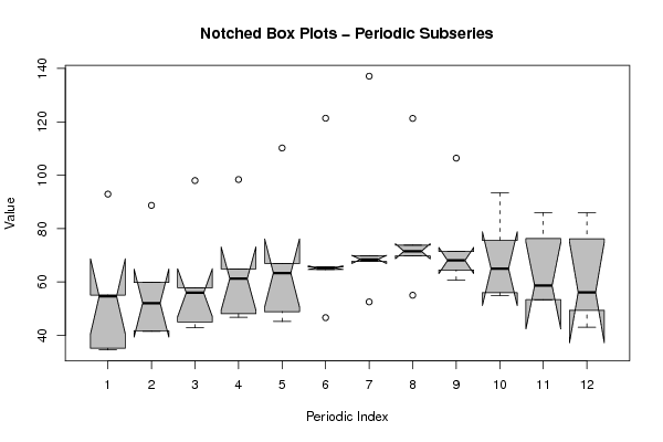
| Title produced by software | Mean Plot | ||||||||||||||||||||
| Date of computation | Sun, 19 Dec 2010 21:32:04 +0000 | ||||||||||||||||||||
| Cite this page as follows | Statistical Computations at FreeStatistics.org, Office for Research Development and Education, URL https://freestatistics.org/blog/index.php?v=date/2010/Dec/19/t12927941990x4b4so2sz0xzq4.htm/, Retrieved Sat, 04 May 2024 23:17:53 +0000 | ||||||||||||||||||||
| Statistical Computations at FreeStatistics.org, Office for Research Development and Education, URL https://freestatistics.org/blog/index.php?pk=112760, Retrieved Sat, 04 May 2024 23:17:53 +0000 | |||||||||||||||||||||
| QR Codes: | |||||||||||||||||||||
|
| |||||||||||||||||||||
| Original text written by user: | |||||||||||||||||||||
| IsPrivate? | No (this computation is public) | ||||||||||||||||||||
| User-defined keywords | |||||||||||||||||||||
| Estimated Impact | 128 | ||||||||||||||||||||
Tree of Dependent Computations | |||||||||||||||||||||
| Family? (F = Feedback message, R = changed R code, M = changed R Module, P = changed Parameters, D = changed Data) | |||||||||||||||||||||
| - [Bivariate Data Series] [Bivariate dataset] [2008-01-05 23:51:08] [74be16979710d4c4e7c6647856088456] - RMPD [Blocked Bootstrap Plot - Central Tendency] [Colombia Coffee] [2008-01-07 10:26:26] [74be16979710d4c4e7c6647856088456] - RMPD [Notched Boxplots] [Notched Boxplot g...] [2010-12-18 19:31:51] [1afa3497b02a8d7c9f6727c1b17b89b2] - RM D [Mean Plot] [Mean Plot gasolie...] [2010-12-18 20:17:33] [1afa3497b02a8d7c9f6727c1b17b89b2] - D [Mean Plot] [Mean Plot Houtskool] [2010-12-18 20:23:05] [1afa3497b02a8d7c9f6727c1b17b89b2] - PD [Mean Plot] [Notched Boxplot O...] [2010-12-19 21:32:04] [214713b86cef2e1efaaf6d85aa84ff3c] [Current] | |||||||||||||||||||||
| Feedback Forum | |||||||||||||||||||||
Post a new message | |||||||||||||||||||||
Dataset | |||||||||||||||||||||
| Dataseries X: | |||||||||||||||||||||
35.16 41.54 45.07 46.84 45.20 46.65 52.55 55.05 60.75 55.99 53.39 49.42 55.12 59.84 55.98 61.27 66.94 64.67 67.74 69.79 64.49 54.92 53.32 56.13 54.63 52.11 57.83 64.93 63.40 65.37 69.91 73.81 71.42 75.57 86.02 85.91 92.93 88.71 98.01 98.39 110.21 121.36 137.11 121.29 106.41 93.38 58.66 43.12 34.57 41.77 42.85 48.09 48.91 65.62 68.47 71.52 68.07 65.00 76.34 76.18 | |||||||||||||||||||||
Tables (Output of Computation) | |||||||||||||||||||||
| |||||||||||||||||||||
Figures (Output of Computation) | |||||||||||||||||||||
Input Parameters & R Code | |||||||||||||||||||||
| Parameters (Session): | |||||||||||||||||||||
| par1 = 12 ; | |||||||||||||||||||||
| Parameters (R input): | |||||||||||||||||||||
| par1 = 12 ; | |||||||||||||||||||||
| R code (references can be found in the software module): | |||||||||||||||||||||
par1 <- as.numeric(par1) | |||||||||||||||||||||