Repository of Reproducible Computations

Free Statistics

of Irreproducible Research!

Author's title

Author

*The author of this computation has been verified*

R Software Module

rwasp_autocorrelation.wasp

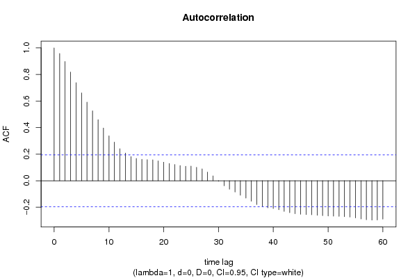
Title produced by software

(Partial) Autocorrelation Function

Date of computation

Sun, 19 Dec 2010 16:55:52 +0000

Cite this page as follows

Statistical Computations at FreeStatistics.org, Office for Research Development and Education, URL https://freestatistics.org/blog/index.php?v=date/2010/Dec/19/t1292777629h6pijgf8rvfpmm8.htm/, Retrieved Sun, 05 May 2024 06:21:18 +0000

Statistical Computations at FreeStatistics.org, Office for Research Development and Education, URL https://freestatistics.org/blog/index.php?pk=112614, Retrieved Sun, 05 May 2024 06:21:18 +0000

QR Codes:

Paste this QR Code to cite your computation.

Original text written by user:

IsPrivate?

No (this computation is public)

User-defined keywords

Estimated Impact

136

Family? (F = Feedback message, R = changed R code, M = changed R Module, P = changed Parameters, D = changed Data)

-     [Bivariate Data Series] [Bivariate dataset] [2008-01-05 23:51:08] [74be16979710d4c4e7c6647856088456]
F RMPD  [Univariate Explorative Data Analysis] [Colombia Coffee] [2008-01-07 14:21:11] [74be16979710d4c4e7c6647856088456]
F RMPD    [Univariate Data Series] [] [2009-10-14 08:30:28] [74be16979710d4c4e7c6647856088456]
- RMP       [Univariate Explorative Data Analysis] [WS3V1-Assumpties] [2009-10-19 09:51:45] [90e6802d28d0afa9b030a19cd25ed2b0]
- R  D        [Univariate Explorative Data Analysis] [WorkShop3 (SHW)] [2009-10-20 21:02:34] [37daf76adc256428993ec4063536c760]
- RM            [(Partial) Autocorrelation Function] [] [2009-10-23 13:34:22] [023d83ebdf42a2acf423907b4076e8a1]
-  MPD              [(Partial) Autocorrelation Function] [] [2010-12-19 16:55:52] [6b31f806e9ccc1f74a26091056f791cb] [Current]

Feedback Forum

Post a new message

Dataseries X:

Download CSV

Histogram

Boxplots

Summary of computational transaction
Raw Input	view raw input (R code)
Raw Output	view raw output of R engine
Computing time	1 seconds
R Server	'RServer@AstonUniversity' @ vre.aston.ac.uk

\begin{tabular}{lllllllll}
\hline
Summary of computational transaction \tabularnewline
Raw Input & view raw input (R code)  \tabularnewline
Raw Output & view raw output of R engine  \tabularnewline
Computing time & 1 seconds \tabularnewline
R Server & 'RServer@AstonUniversity' @ vre.aston.ac.uk \tabularnewline
\hline
\end{tabular}
%Source: https://freestatistics.org/blog/index.php?pk=112614&T=0

[TABLE]
[ROW][C]Summary of computational transaction[/C][/ROW]
[ROW][C]Raw Input[/C][C]view raw input (R code) [/C][/ROW]
[ROW][C]Raw Output[/C][C]view raw output of R engine [/C][/ROW]
[ROW][C]Computing time[/C][C]1 seconds[/C][/ROW]
[ROW][C]R Server[/C][C]'RServer@AstonUniversity' @ vre.aston.ac.uk[/C][/ROW]
[/TABLE]
Source: https://freestatistics.org/blog/index.php?pk=112614&T=0

Globally Unique Identifier (entire table): ba.freestatistics.org/blog/index.php?pk=112614&T=0

As an alternative you can also use a QR Code:

The GUIDs for individual cells are displayed in the table below:

Summary of computational transaction
Raw Input	view raw input (R code)
Raw Output	view raw output of R engine
Computing time	1 seconds
R Server	'RServer@AstonUniversity' @ vre.aston.ac.uk

Autocorrelation Function
Time lag k	ACF(k)	T-STAT	P-value
1	0.957675	9.6245	0
2	0.897589	9.0207	0
3	0.817532	8.2161	0
4	0.738489	7.4217	0
5	0.660657	6.6395	0
6	0.592007	5.9496	0
7	0.525772	5.2839	0
8	0.459861	4.6215	6e-06
9	0.396537	3.9851	6.4e-05
10	0.337541	3.3922	0.000495
11	0.290567	2.9202	0.002157
12	0.240986	2.4219	0.008612
13	0.208076	2.0911	0.019512
14	0.181575	1.8248	0.035493
15	0.167654	1.6849	0.047548
16	0.161063	1.6187	0.05432
17	0.158213	1.59	0.057478
18	0.15711	1.5789	0.058739
19	0.149833	1.5058	0.06762
20	0.139718	1.4041	0.081671
21	0.129987	1.3064	0.0972
22	0.12241	1.2302	0.110738
23	0.113778	1.1435	0.127777
24	0.109345	1.0989	0.137212
25	0.109899	1.1045	0.136006
26	0.101168	1.0167	0.155856
27	0.089346	0.8979	0.185684
28	0.06508	0.654	0.257285
29	0.036211	0.3639	0.358342
30	-0.003826	-0.0385	0.484701
31	-0.038287	-0.3848	0.350605
32	-0.064222	-0.6454	0.260059
33	-0.084829	-0.8525	0.197972
34	-0.109255	-1.098	0.137409
35	-0.131342	-1.32	0.094915
36	-0.154055	-1.5482	0.062348
37	-0.17894	-1.7983	0.037556
38	-0.193992	-1.9496	0.026999
39	-0.203685	-2.047	0.021627
40	-0.209126	-2.1017	0.019034
41	-0.218574	-2.1966	0.015166
42	-0.23088	-2.3203	0.011167
43	-0.240967	-2.4217	0.008616
44	-0.248386	-2.4963	0.007085
45	-0.252727	-2.5399	0.006306
46	-0.25549	-2.5676	0.005852
47	-0.256018	-2.5729	0.005769
48	-0.260504	-2.618	0.005102
49	-0.263397	-2.6471	0.00471
50	-0.265644	-2.6697	0.004424
51	-0.267326	-2.6866	0.004221
52	-0.268146	-2.6948	0.004125
53	-0.270734	-2.7208	0.003835
54	-0.273101	-2.7446	0.003585
55	-0.279884	-2.8128	0.002951
56	-0.287934	-2.8937	0.002332
57	-0.293751	-2.9522	0.001962
58	-0.296364	-2.9784	0.001814
59	-0.295453	-2.9693	0.001864
60	-0.289219	-2.9066	0.002246

\begin{tabular}{lllllllll}
\hline
Autocorrelation Function \tabularnewline
Time lag k & ACF(k) & T-STAT & P-value \tabularnewline
1 & 0.957675 & 9.6245 & 0 \tabularnewline
2 & 0.897589 & 9.0207 & 0 \tabularnewline
3 & 0.817532 & 8.2161 & 0 \tabularnewline
4 & 0.738489 & 7.4217 & 0 \tabularnewline
5 & 0.660657 & 6.6395 & 0 \tabularnewline
6 & 0.592007 & 5.9496 & 0 \tabularnewline
7 & 0.525772 & 5.2839 & 0 \tabularnewline
8 & 0.459861 & 4.6215 & 6e-06 \tabularnewline
9 & 0.396537 & 3.9851 & 6.4e-05 \tabularnewline
10 & 0.337541 & 3.3922 & 0.000495 \tabularnewline
11 & 0.290567 & 2.9202 & 0.002157 \tabularnewline
12 & 0.240986 & 2.4219 & 0.008612 \tabularnewline
13 & 0.208076 & 2.0911 & 0.019512 \tabularnewline
14 & 0.181575 & 1.8248 & 0.035493 \tabularnewline
15 & 0.167654 & 1.6849 & 0.047548 \tabularnewline
16 & 0.161063 & 1.6187 & 0.05432 \tabularnewline
17 & 0.158213 & 1.59 & 0.057478 \tabularnewline
18 & 0.15711 & 1.5789 & 0.058739 \tabularnewline
19 & 0.149833 & 1.5058 & 0.06762 \tabularnewline
20 & 0.139718 & 1.4041 & 0.081671 \tabularnewline
21 & 0.129987 & 1.3064 & 0.0972 \tabularnewline
22 & 0.12241 & 1.2302 & 0.110738 \tabularnewline
23 & 0.113778 & 1.1435 & 0.127777 \tabularnewline
24 & 0.109345 & 1.0989 & 0.137212 \tabularnewline
25 & 0.109899 & 1.1045 & 0.136006 \tabularnewline
26 & 0.101168 & 1.0167 & 0.155856 \tabularnewline
27 & 0.089346 & 0.8979 & 0.185684 \tabularnewline
28 & 0.06508 & 0.654 & 0.257285 \tabularnewline
29 & 0.036211 & 0.3639 & 0.358342 \tabularnewline
30 & -0.003826 & -0.0385 & 0.484701 \tabularnewline
31 & -0.038287 & -0.3848 & 0.350605 \tabularnewline
32 & -0.064222 & -0.6454 & 0.260059 \tabularnewline
33 & -0.084829 & -0.8525 & 0.197972 \tabularnewline
34 & -0.109255 & -1.098 & 0.137409 \tabularnewline
35 & -0.131342 & -1.32 & 0.094915 \tabularnewline
36 & -0.154055 & -1.5482 & 0.062348 \tabularnewline
37 & -0.17894 & -1.7983 & 0.037556 \tabularnewline
38 & -0.193992 & -1.9496 & 0.026999 \tabularnewline
39 & -0.203685 & -2.047 & 0.021627 \tabularnewline
40 & -0.209126 & -2.1017 & 0.019034 \tabularnewline
41 & -0.218574 & -2.1966 & 0.015166 \tabularnewline
42 & -0.23088 & -2.3203 & 0.011167 \tabularnewline
43 & -0.240967 & -2.4217 & 0.008616 \tabularnewline
44 & -0.248386 & -2.4963 & 0.007085 \tabularnewline
45 & -0.252727 & -2.5399 & 0.006306 \tabularnewline
46 & -0.25549 & -2.5676 & 0.005852 \tabularnewline
47 & -0.256018 & -2.5729 & 0.005769 \tabularnewline
48 & -0.260504 & -2.618 & 0.005102 \tabularnewline
49 & -0.263397 & -2.6471 & 0.00471 \tabularnewline
50 & -0.265644 & -2.6697 & 0.004424 \tabularnewline
51 & -0.267326 & -2.6866 & 0.004221 \tabularnewline
52 & -0.268146 & -2.6948 & 0.004125 \tabularnewline
53 & -0.270734 & -2.7208 & 0.003835 \tabularnewline
54 & -0.273101 & -2.7446 & 0.003585 \tabularnewline
55 & -0.279884 & -2.8128 & 0.002951 \tabularnewline
56 & -0.287934 & -2.8937 & 0.002332 \tabularnewline
57 & -0.293751 & -2.9522 & 0.001962 \tabularnewline
58 & -0.296364 & -2.9784 & 0.001814 \tabularnewline
59 & -0.295453 & -2.9693 & 0.001864 \tabularnewline
60 & -0.289219 & -2.9066 & 0.002246 \tabularnewline
\hline
\end{tabular}
%Source: https://freestatistics.org/blog/index.php?pk=112614&T=1

[TABLE]
[ROW][C]Autocorrelation Function[/C][/ROW]
[ROW][C]Time lag k[/C][C]ACF(k)[/C][C]T-STAT[/C][C]P-value[/C][/ROW]
[ROW][C]1[/C][C]0.957675[/C][C]9.6245[/C][C]0[/C][/ROW]
[ROW][C]2[/C][C]0.897589[/C][C]9.0207[/C][C]0[/C][/ROW]
[ROW][C]3[/C][C]0.817532[/C][C]8.2161[/C][C]0[/C][/ROW]
[ROW][C]4[/C][C]0.738489[/C][C]7.4217[/C][C]0[/C][/ROW]
[ROW][C]5[/C][C]0.660657[/C][C]6.6395[/C][C]0[/C][/ROW]
[ROW][C]6[/C][C]0.592007[/C][C]5.9496[/C][C]0[/C][/ROW]
[ROW][C]7[/C][C]0.525772[/C][C]5.2839[/C][C]0[/C][/ROW]
[ROW][C]8[/C][C]0.459861[/C][C]4.6215[/C][C]6e-06[/C][/ROW]
[ROW][C]9[/C][C]0.396537[/C][C]3.9851[/C][C]6.4e-05[/C][/ROW]
[ROW][C]10[/C][C]0.337541[/C][C]3.3922[/C][C]0.000495[/C][/ROW]
[ROW][C]11[/C][C]0.290567[/C][C]2.9202[/C][C]0.002157[/C][/ROW]
[ROW][C]12[/C][C]0.240986[/C][C]2.4219[/C][C]0.008612[/C][/ROW]
[ROW][C]13[/C][C]0.208076[/C][C]2.0911[/C][C]0.019512[/C][/ROW]
[ROW][C]14[/C][C]0.181575[/C][C]1.8248[/C][C]0.035493[/C][/ROW]
[ROW][C]15[/C][C]0.167654[/C][C]1.6849[/C][C]0.047548[/C][/ROW]
[ROW][C]16[/C][C]0.161063[/C][C]1.6187[/C][C]0.05432[/C][/ROW]
[ROW][C]17[/C][C]0.158213[/C][C]1.59[/C][C]0.057478[/C][/ROW]
[ROW][C]18[/C][C]0.15711[/C][C]1.5789[/C][C]0.058739[/C][/ROW]
[ROW][C]19[/C][C]0.149833[/C][C]1.5058[/C][C]0.06762[/C][/ROW]
[ROW][C]20[/C][C]0.139718[/C][C]1.4041[/C][C]0.081671[/C][/ROW]
[ROW][C]21[/C][C]0.129987[/C][C]1.3064[/C][C]0.0972[/C][/ROW]
[ROW][C]22[/C][C]0.12241[/C][C]1.2302[/C][C]0.110738[/C][/ROW]
[ROW][C]23[/C][C]0.113778[/C][C]1.1435[/C][C]0.127777[/C][/ROW]
[ROW][C]24[/C][C]0.109345[/C][C]1.0989[/C][C]0.137212[/C][/ROW]
[ROW][C]25[/C][C]0.109899[/C][C]1.1045[/C][C]0.136006[/C][/ROW]
[ROW][C]26[/C][C]0.101168[/C][C]1.0167[/C][C]0.155856[/C][/ROW]
[ROW][C]27[/C][C]0.089346[/C][C]0.8979[/C][C]0.185684[/C][/ROW]
[ROW][C]28[/C][C]0.06508[/C][C]0.654[/C][C]0.257285[/C][/ROW]
[ROW][C]29[/C][C]0.036211[/C][C]0.3639[/C][C]0.358342[/C][/ROW]
[ROW][C]30[/C][C]-0.003826[/C][C]-0.0385[/C][C]0.484701[/C][/ROW]
[ROW][C]31[/C][C]-0.038287[/C][C]-0.3848[/C][C]0.350605[/C][/ROW]
[ROW][C]32[/C][C]-0.064222[/C][C]-0.6454[/C][C]0.260059[/C][/ROW]
[ROW][C]33[/C][C]-0.084829[/C][C]-0.8525[/C][C]0.197972[/C][/ROW]
[ROW][C]34[/C][C]-0.109255[/C][C]-1.098[/C][C]0.137409[/C][/ROW]
[ROW][C]35[/C][C]-0.131342[/C][C]-1.32[/C][C]0.094915[/C][/ROW]
[ROW][C]36[/C][C]-0.154055[/C][C]-1.5482[/C][C]0.062348[/C][/ROW]
[ROW][C]37[/C][C]-0.17894[/C][C]-1.7983[/C][C]0.037556[/C][/ROW]
[ROW][C]38[/C][C]-0.193992[/C][C]-1.9496[/C][C]0.026999[/C][/ROW]
[ROW][C]39[/C][C]-0.203685[/C][C]-2.047[/C][C]0.021627[/C][/ROW]
[ROW][C]40[/C][C]-0.209126[/C][C]-2.1017[/C][C]0.019034[/C][/ROW]
[ROW][C]41[/C][C]-0.218574[/C][C]-2.1966[/C][C]0.015166[/C][/ROW]
[ROW][C]42[/C][C]-0.23088[/C][C]-2.3203[/C][C]0.011167[/C][/ROW]
[ROW][C]43[/C][C]-0.240967[/C][C]-2.4217[/C][C]0.008616[/C][/ROW]
[ROW][C]44[/C][C]-0.248386[/C][C]-2.4963[/C][C]0.007085[/C][/ROW]
[ROW][C]45[/C][C]-0.252727[/C][C]-2.5399[/C][C]0.006306[/C][/ROW]
[ROW][C]46[/C][C]-0.25549[/C][C]-2.5676[/C][C]0.005852[/C][/ROW]
[ROW][C]47[/C][C]-0.256018[/C][C]-2.5729[/C][C]0.005769[/C][/ROW]
[ROW][C]48[/C][C]-0.260504[/C][C]-2.618[/C][C]0.005102[/C][/ROW]
[ROW][C]49[/C][C]-0.263397[/C][C]-2.6471[/C][C]0.00471[/C][/ROW]
[ROW][C]50[/C][C]-0.265644[/C][C]-2.6697[/C][C]0.004424[/C][/ROW]
[ROW][C]51[/C][C]-0.267326[/C][C]-2.6866[/C][C]0.004221[/C][/ROW]
[ROW][C]52[/C][C]-0.268146[/C][C]-2.6948[/C][C]0.004125[/C][/ROW]
[ROW][C]53[/C][C]-0.270734[/C][C]-2.7208[/C][C]0.003835[/C][/ROW]
[ROW][C]54[/C][C]-0.273101[/C][C]-2.7446[/C][C]0.003585[/C][/ROW]
[ROW][C]55[/C][C]-0.279884[/C][C]-2.8128[/C][C]0.002951[/C][/ROW]
[ROW][C]56[/C][C]-0.287934[/C][C]-2.8937[/C][C]0.002332[/C][/ROW]
[ROW][C]57[/C][C]-0.293751[/C][C]-2.9522[/C][C]0.001962[/C][/ROW]
[ROW][C]58[/C][C]-0.296364[/C][C]-2.9784[/C][C]0.001814[/C][/ROW]
[ROW][C]59[/C][C]-0.295453[/C][C]-2.9693[/C][C]0.001864[/C][/ROW]
[ROW][C]60[/C][C]-0.289219[/C][C]-2.9066[/C][C]0.002246[/C][/ROW]
[/TABLE]
Source: https://freestatistics.org/blog/index.php?pk=112614&T=1

Globally Unique Identifier (entire table): ba.freestatistics.org/blog/index.php?pk=112614&T=1

As an alternative you can also use a QR Code:

The GUIDs for individual cells are displayed in the table below:

Autocorrelation Function
Time lag k	ACF(k)	T-STAT	P-value
1	0.957675	9.6245	0
2	0.897589	9.0207	0
3	0.817532	8.2161	0
4	0.738489	7.4217	0
5	0.660657	6.6395	0
6	0.592007	5.9496	0
7	0.525772	5.2839	0
8	0.459861	4.6215	6e-06
9	0.396537	3.9851	6.4e-05
10	0.337541	3.3922	0.000495
11	0.290567	2.9202	0.002157
12	0.240986	2.4219	0.008612
13	0.208076	2.0911	0.019512
14	0.181575	1.8248	0.035493
15	0.167654	1.6849	0.047548
16	0.161063	1.6187	0.05432
17	0.158213	1.59	0.057478
18	0.15711	1.5789	0.058739
19	0.149833	1.5058	0.06762
20	0.139718	1.4041	0.081671
21	0.129987	1.3064	0.0972
22	0.12241	1.2302	0.110738
23	0.113778	1.1435	0.127777
24	0.109345	1.0989	0.137212
25	0.109899	1.1045	0.136006
26	0.101168	1.0167	0.155856
27	0.089346	0.8979	0.185684
28	0.06508	0.654	0.257285
29	0.036211	0.3639	0.358342
30	-0.003826	-0.0385	0.484701
31	-0.038287	-0.3848	0.350605
32	-0.064222	-0.6454	0.260059
33	-0.084829	-0.8525	0.197972
34	-0.109255	-1.098	0.137409
35	-0.131342	-1.32	0.094915
36	-0.154055	-1.5482	0.062348
37	-0.17894	-1.7983	0.037556
38	-0.193992	-1.9496	0.026999
39	-0.203685	-2.047	0.021627
40	-0.209126	-2.1017	0.019034
41	-0.218574	-2.1966	0.015166
42	-0.23088	-2.3203	0.011167
43	-0.240967	-2.4217	0.008616
44	-0.248386	-2.4963	0.007085
45	-0.252727	-2.5399	0.006306
46	-0.25549	-2.5676	0.005852
47	-0.256018	-2.5729	0.005769
48	-0.260504	-2.618	0.005102
49	-0.263397	-2.6471	0.00471
50	-0.265644	-2.6697	0.004424
51	-0.267326	-2.6866	0.004221
52	-0.268146	-2.6948	0.004125
53	-0.270734	-2.7208	0.003835
54	-0.273101	-2.7446	0.003585
55	-0.279884	-2.8128	0.002951
56	-0.287934	-2.8937	0.002332
57	-0.293751	-2.9522	0.001962
58	-0.296364	-2.9784	0.001814
59	-0.295453	-2.9693	0.001864
60	-0.289219	-2.9066	0.002246

Partial Autocorrelation Function
Time lag k	PACF(k)	T-STAT	P-value
1	0.957675	9.6245	0
2	-0.235965	-2.3714	0.009808
3	-0.241857	-2.4306	0.008418
4	0.053416	0.5368	0.296286
5	0.002209	0.0222	0.491166
6	0.038267	0.3846	0.35068
7	-0.058933	-0.5923	0.277496
8	-0.087708	-0.8815	0.190082
9	0.003801	0.0382	0.484801
10	0.016907	0.1699	0.432708
11	0.092058	0.9252	0.178541
12	-0.15043	-1.5118	0.066853
13	0.145746	1.4647	0.07305
14	0.037422	0.3761	0.353822
15	0.040246	0.4045	0.343363
16	0.043657	0.4387	0.330891
17	-0.061277	-0.6158	0.269698
18	0.01977	0.1987	0.421454
19	-0.081364	-0.8177	0.207728
20	-0.011862	-0.1192	0.452674
21	0.051462	0.5172	0.303077
22	-0.016508	-0.1659	0.434283
23	0.007485	0.0752	0.470095
24	0.001859	0.0187	0.492565
25	0.102707	1.0322	0.152225
26	-0.173057	-1.7392	0.042523
27	-0.008299	-0.0834	0.466847
28	-0.091354	-0.9181	0.180378
29	-0.045478	-0.457	0.324309
30	-0.06071	-0.6101	0.271574
31	0.050267	0.5052	0.307268
32	0.096782	0.9727	0.166525
33	-0.070819	-0.7117	0.239139
34	-0.123554	-1.2417	0.108612
35	0.034453	0.3462	0.36494
36	-0.027059	-0.2719	0.393112
37	0.007938	0.0798	0.468286
38	0.047816	0.4805	0.315939
39	0.017573	0.1766	0.430086
40	-0.103536	-1.0405	0.150291
41	-0.069095	-0.6944	0.244514
42	-0.082004	-0.8241	0.205903
43	0.02732	0.2746	0.392105
44	0.040831	0.4103	0.341211
45	0.016009	0.1609	0.43625
46	-0.04779	-0.4803	0.316033
47	0.016562	0.1664	0.43407
48	-0.044764	-0.4499	0.326884
49	-0.014817	-0.1489	0.440962
50	-0.034718	-0.3489	0.363942
51	-0.029167	-0.2931	0.385015
52	0.02254	0.2265	0.410625
53	-0.016837	-0.1692	0.432985
54	-0.054141	-0.5441	0.293783
55	-0.011185	-0.1124	0.455362
56	-0.048224	-0.4846	0.314489
57	0.031877	0.3204	0.37468
58	-0.016335	-0.1642	0.434966
59	0.073678	0.7405	0.230371
60	-0.021005	-0.2111	0.416617

\begin{tabular}{lllllllll}
\hline
Partial Autocorrelation Function \tabularnewline
Time lag k & PACF(k) & T-STAT & P-value \tabularnewline
1 & 0.957675 & 9.6245 & 0 \tabularnewline
2 & -0.235965 & -2.3714 & 0.009808 \tabularnewline
3 & -0.241857 & -2.4306 & 0.008418 \tabularnewline
4 & 0.053416 & 0.5368 & 0.296286 \tabularnewline
5 & 0.002209 & 0.0222 & 0.491166 \tabularnewline
6 & 0.038267 & 0.3846 & 0.35068 \tabularnewline
7 & -0.058933 & -0.5923 & 0.277496 \tabularnewline
8 & -0.087708 & -0.8815 & 0.190082 \tabularnewline
9 & 0.003801 & 0.0382 & 0.484801 \tabularnewline
10 & 0.016907 & 0.1699 & 0.432708 \tabularnewline
11 & 0.092058 & 0.9252 & 0.178541 \tabularnewline
12 & -0.15043 & -1.5118 & 0.066853 \tabularnewline
13 & 0.145746 & 1.4647 & 0.07305 \tabularnewline
14 & 0.037422 & 0.3761 & 0.353822 \tabularnewline
15 & 0.040246 & 0.4045 & 0.343363 \tabularnewline
16 & 0.043657 & 0.4387 & 0.330891 \tabularnewline
17 & -0.061277 & -0.6158 & 0.269698 \tabularnewline
18 & 0.01977 & 0.1987 & 0.421454 \tabularnewline
19 & -0.081364 & -0.8177 & 0.207728 \tabularnewline
20 & -0.011862 & -0.1192 & 0.452674 \tabularnewline
21 & 0.051462 & 0.5172 & 0.303077 \tabularnewline
22 & -0.016508 & -0.1659 & 0.434283 \tabularnewline
23 & 0.007485 & 0.0752 & 0.470095 \tabularnewline
24 & 0.001859 & 0.0187 & 0.492565 \tabularnewline
25 & 0.102707 & 1.0322 & 0.152225 \tabularnewline
26 & -0.173057 & -1.7392 & 0.042523 \tabularnewline
27 & -0.008299 & -0.0834 & 0.466847 \tabularnewline
28 & -0.091354 & -0.9181 & 0.180378 \tabularnewline
29 & -0.045478 & -0.457 & 0.324309 \tabularnewline
30 & -0.06071 & -0.6101 & 0.271574 \tabularnewline
31 & 0.050267 & 0.5052 & 0.307268 \tabularnewline
32 & 0.096782 & 0.9727 & 0.166525 \tabularnewline
33 & -0.070819 & -0.7117 & 0.239139 \tabularnewline
34 & -0.123554 & -1.2417 & 0.108612 \tabularnewline
35 & 0.034453 & 0.3462 & 0.36494 \tabularnewline
36 & -0.027059 & -0.2719 & 0.393112 \tabularnewline
37 & 0.007938 & 0.0798 & 0.468286 \tabularnewline
38 & 0.047816 & 0.4805 & 0.315939 \tabularnewline
39 & 0.017573 & 0.1766 & 0.430086 \tabularnewline
40 & -0.103536 & -1.0405 & 0.150291 \tabularnewline
41 & -0.069095 & -0.6944 & 0.244514 \tabularnewline
42 & -0.082004 & -0.8241 & 0.205903 \tabularnewline
43 & 0.02732 & 0.2746 & 0.392105 \tabularnewline
44 & 0.040831 & 0.4103 & 0.341211 \tabularnewline
45 & 0.016009 & 0.1609 & 0.43625 \tabularnewline
46 & -0.04779 & -0.4803 & 0.316033 \tabularnewline
47 & 0.016562 & 0.1664 & 0.43407 \tabularnewline
48 & -0.044764 & -0.4499 & 0.326884 \tabularnewline
49 & -0.014817 & -0.1489 & 0.440962 \tabularnewline
50 & -0.034718 & -0.3489 & 0.363942 \tabularnewline
51 & -0.029167 & -0.2931 & 0.385015 \tabularnewline
52 & 0.02254 & 0.2265 & 0.410625 \tabularnewline
53 & -0.016837 & -0.1692 & 0.432985 \tabularnewline
54 & -0.054141 & -0.5441 & 0.293783 \tabularnewline
55 & -0.011185 & -0.1124 & 0.455362 \tabularnewline
56 & -0.048224 & -0.4846 & 0.314489 \tabularnewline
57 & 0.031877 & 0.3204 & 0.37468 \tabularnewline
58 & -0.016335 & -0.1642 & 0.434966 \tabularnewline
59 & 0.073678 & 0.7405 & 0.230371 \tabularnewline
60 & -0.021005 & -0.2111 & 0.416617 \tabularnewline
\hline
\end{tabular}
%Source: https://freestatistics.org/blog/index.php?pk=112614&T=2

[TABLE]
[ROW][C]Partial Autocorrelation Function[/C][/ROW]
[ROW][C]Time lag k[/C][C]PACF(k)[/C][C]T-STAT[/C][C]P-value[/C][/ROW]
[ROW][C]1[/C][C]0.957675[/C][C]9.6245[/C][C]0[/C][/ROW]
[ROW][C]2[/C][C]-0.235965[/C][C]-2.3714[/C][C]0.009808[/C][/ROW]
[ROW][C]3[/C][C]-0.241857[/C][C]-2.4306[/C][C]0.008418[/C][/ROW]
[ROW][C]4[/C][C]0.053416[/C][C]0.5368[/C][C]0.296286[/C][/ROW]
[ROW][C]5[/C][C]0.002209[/C][C]0.0222[/C][C]0.491166[/C][/ROW]
[ROW][C]6[/C][C]0.038267[/C][C]0.3846[/C][C]0.35068[/C][/ROW]
[ROW][C]7[/C][C]-0.058933[/C][C]-0.5923[/C][C]0.277496[/C][/ROW]
[ROW][C]8[/C][C]-0.087708[/C][C]-0.8815[/C][C]0.190082[/C][/ROW]
[ROW][C]9[/C][C]0.003801[/C][C]0.0382[/C][C]0.484801[/C][/ROW]
[ROW][C]10[/C][C]0.016907[/C][C]0.1699[/C][C]0.432708[/C][/ROW]
[ROW][C]11[/C][C]0.092058[/C][C]0.9252[/C][C]0.178541[/C][/ROW]
[ROW][C]12[/C][C]-0.15043[/C][C]-1.5118[/C][C]0.066853[/C][/ROW]
[ROW][C]13[/C][C]0.145746[/C][C]1.4647[/C][C]0.07305[/C][/ROW]
[ROW][C]14[/C][C]0.037422[/C][C]0.3761[/C][C]0.353822[/C][/ROW]
[ROW][C]15[/C][C]0.040246[/C][C]0.4045[/C][C]0.343363[/C][/ROW]
[ROW][C]16[/C][C]0.043657[/C][C]0.4387[/C][C]0.330891[/C][/ROW]
[ROW][C]17[/C][C]-0.061277[/C][C]-0.6158[/C][C]0.269698[/C][/ROW]
[ROW][C]18[/C][C]0.01977[/C][C]0.1987[/C][C]0.421454[/C][/ROW]
[ROW][C]19[/C][C]-0.081364[/C][C]-0.8177[/C][C]0.207728[/C][/ROW]
[ROW][C]20[/C][C]-0.011862[/C][C]-0.1192[/C][C]0.452674[/C][/ROW]
[ROW][C]21[/C][C]0.051462[/C][C]0.5172[/C][C]0.303077[/C][/ROW]
[ROW][C]22[/C][C]-0.016508[/C][C]-0.1659[/C][C]0.434283[/C][/ROW]
[ROW][C]23[/C][C]0.007485[/C][C]0.0752[/C][C]0.470095[/C][/ROW]
[ROW][C]24[/C][C]0.001859[/C][C]0.0187[/C][C]0.492565[/C][/ROW]
[ROW][C]25[/C][C]0.102707[/C][C]1.0322[/C][C]0.152225[/C][/ROW]
[ROW][C]26[/C][C]-0.173057[/C][C]-1.7392[/C][C]0.042523[/C][/ROW]
[ROW][C]27[/C][C]-0.008299[/C][C]-0.0834[/C][C]0.466847[/C][/ROW]
[ROW][C]28[/C][C]-0.091354[/C][C]-0.9181[/C][C]0.180378[/C][/ROW]
[ROW][C]29[/C][C]-0.045478[/C][C]-0.457[/C][C]0.324309[/C][/ROW]
[ROW][C]30[/C][C]-0.06071[/C][C]-0.6101[/C][C]0.271574[/C][/ROW]
[ROW][C]31[/C][C]0.050267[/C][C]0.5052[/C][C]0.307268[/C][/ROW]
[ROW][C]32[/C][C]0.096782[/C][C]0.9727[/C][C]0.166525[/C][/ROW]
[ROW][C]33[/C][C]-0.070819[/C][C]-0.7117[/C][C]0.239139[/C][/ROW]
[ROW][C]34[/C][C]-0.123554[/C][C]-1.2417[/C][C]0.108612[/C][/ROW]
[ROW][C]35[/C][C]0.034453[/C][C]0.3462[/C][C]0.36494[/C][/ROW]
[ROW][C]36[/C][C]-0.027059[/C][C]-0.2719[/C][C]0.393112[/C][/ROW]
[ROW][C]37[/C][C]0.007938[/C][C]0.0798[/C][C]0.468286[/C][/ROW]
[ROW][C]38[/C][C]0.047816[/C][C]0.4805[/C][C]0.315939[/C][/ROW]
[ROW][C]39[/C][C]0.017573[/C][C]0.1766[/C][C]0.430086[/C][/ROW]
[ROW][C]40[/C][C]-0.103536[/C][C]-1.0405[/C][C]0.150291[/C][/ROW]
[ROW][C]41[/C][C]-0.069095[/C][C]-0.6944[/C][C]0.244514[/C][/ROW]
[ROW][C]42[/C][C]-0.082004[/C][C]-0.8241[/C][C]0.205903[/C][/ROW]
[ROW][C]43[/C][C]0.02732[/C][C]0.2746[/C][C]0.392105[/C][/ROW]
[ROW][C]44[/C][C]0.040831[/C][C]0.4103[/C][C]0.341211[/C][/ROW]
[ROW][C]45[/C][C]0.016009[/C][C]0.1609[/C][C]0.43625[/C][/ROW]
[ROW][C]46[/C][C]-0.04779[/C][C]-0.4803[/C][C]0.316033[/C][/ROW]
[ROW][C]47[/C][C]0.016562[/C][C]0.1664[/C][C]0.43407[/C][/ROW]
[ROW][C]48[/C][C]-0.044764[/C][C]-0.4499[/C][C]0.326884[/C][/ROW]
[ROW][C]49[/C][C]-0.014817[/C][C]-0.1489[/C][C]0.440962[/C][/ROW]
[ROW][C]50[/C][C]-0.034718[/C][C]-0.3489[/C][C]0.363942[/C][/ROW]
[ROW][C]51[/C][C]-0.029167[/C][C]-0.2931[/C][C]0.385015[/C][/ROW]
[ROW][C]52[/C][C]0.02254[/C][C]0.2265[/C][C]0.410625[/C][/ROW]
[ROW][C]53[/C][C]-0.016837[/C][C]-0.1692[/C][C]0.432985[/C][/ROW]
[ROW][C]54[/C][C]-0.054141[/C][C]-0.5441[/C][C]0.293783[/C][/ROW]
[ROW][C]55[/C][C]-0.011185[/C][C]-0.1124[/C][C]0.455362[/C][/ROW]
[ROW][C]56[/C][C]-0.048224[/C][C]-0.4846[/C][C]0.314489[/C][/ROW]
[ROW][C]57[/C][C]0.031877[/C][C]0.3204[/C][C]0.37468[/C][/ROW]
[ROW][C]58[/C][C]-0.016335[/C][C]-0.1642[/C][C]0.434966[/C][/ROW]
[ROW][C]59[/C][C]0.073678[/C][C]0.7405[/C][C]0.230371[/C][/ROW]
[ROW][C]60[/C][C]-0.021005[/C][C]-0.2111[/C][C]0.416617[/C][/ROW]
[/TABLE]
Source: https://freestatistics.org/blog/index.php?pk=112614&T=2

Globally Unique Identifier (entire table): ba.freestatistics.org/blog/index.php?pk=112614&T=2

As an alternative you can also use a QR Code:

The GUIDs for individual cells are displayed in the table below:

Partial Autocorrelation Function
Time lag k	PACF(k)	T-STAT	P-value
1	0.957675	9.6245	0
2	-0.235965	-2.3714	0.009808
3	-0.241857	-2.4306	0.008418
4	0.053416	0.5368	0.296286
5	0.002209	0.0222	0.491166
6	0.038267	0.3846	0.35068
7	-0.058933	-0.5923	0.277496
8	-0.087708	-0.8815	0.190082
9	0.003801	0.0382	0.484801
10	0.016907	0.1699	0.432708
11	0.092058	0.9252	0.178541
12	-0.15043	-1.5118	0.066853
13	0.145746	1.4647	0.07305
14	0.037422	0.3761	0.353822
15	0.040246	0.4045	0.343363
16	0.043657	0.4387	0.330891
17	-0.061277	-0.6158	0.269698
18	0.01977	0.1987	0.421454
19	-0.081364	-0.8177	0.207728
20	-0.011862	-0.1192	0.452674
21	0.051462	0.5172	0.303077
22	-0.016508	-0.1659	0.434283
23	0.007485	0.0752	0.470095
24	0.001859	0.0187	0.492565
25	0.102707	1.0322	0.152225
26	-0.173057	-1.7392	0.042523
27	-0.008299	-0.0834	0.466847
28	-0.091354	-0.9181	0.180378
29	-0.045478	-0.457	0.324309
30	-0.06071	-0.6101	0.271574
31	0.050267	0.5052	0.307268
32	0.096782	0.9727	0.166525
33	-0.070819	-0.7117	0.239139
34	-0.123554	-1.2417	0.108612
35	0.034453	0.3462	0.36494
36	-0.027059	-0.2719	0.393112
37	0.007938	0.0798	0.468286
38	0.047816	0.4805	0.315939
39	0.017573	0.1766	0.430086
40	-0.103536	-1.0405	0.150291
41	-0.069095	-0.6944	0.244514
42	-0.082004	-0.8241	0.205903
43	0.02732	0.2746	0.392105
44	0.040831	0.4103	0.341211
45	0.016009	0.1609	0.43625
46	-0.04779	-0.4803	0.316033
47	0.016562	0.1664	0.43407
48	-0.044764	-0.4499	0.326884
49	-0.014817	-0.1489	0.440962
50	-0.034718	-0.3489	0.363942
51	-0.029167	-0.2931	0.385015
52	0.02254	0.2265	0.410625
53	-0.016837	-0.1692	0.432985
54	-0.054141	-0.5441	0.293783
55	-0.011185	-0.1124	0.455362
56	-0.048224	-0.4846	0.314489
57	0.031877	0.3204	0.37468
58	-0.016335	-0.1642	0.434966
59	0.073678	0.7405	0.230371
60	-0.021005	-0.2111	0.416617

Figure 1

PNG link

Postscript link

PDF link

Figure 2

PNG link

Postscript link

PDF link

Parameters (Session):

par1 = 60 ; par2 = 1 ; par3 = 0 ; par4 = 0 ; par5 = 12 ; par6 = White Noise ; par7 = 0.95 ;

Parameters (R input):

par1 = 60 ; par2 = 1 ; par3 = 0 ; par4 = 0 ; par5 = 12 ; par6 = White Noise ; par7 = 0.95 ; par8 = ;

R code (references can be found in the software module):

if (par1 == 'Default') {
par1 = 10*log10(length(x))
} else {
par1 <- as.numeric(par1)
}
par2 <- as.numeric(par2)
par3 <- as.numeric(par3)
par4 <- as.numeric(par4)
par5 <- as.numeric(par5)
if (par6 == 'White Noise') par6 <- 'white' else par6 <- 'ma'
par7 <- as.numeric(par7)
if (par2 == 0) {
x <- log(x)
} else {
x <- (x ^ par2 - 1) / par2
}
if (par3 > 0) x <- diff(x,lag=1,difference=par3)
if (par4 > 0) x <- diff(x,lag=par5,difference=par4)
bitmap(file='pic1.png')
racf <- acf(x, par1, main='Autocorrelation', xlab='time lag', ylab='ACF', ci.type=par6, ci=par7, sub=paste('(lambda=',par2,', d=',par3,', D=',par4,', CI=', par7, ', CI type=',par6,')',sep=''))
dev.off()
bitmap(file='pic2.png')
rpacf <- pacf(x,par1,main='Partial Autocorrelation',xlab='lags',ylab='PACF')
dev.off()
(myacf <- c(racf$acf))
(mypacf <- c(rpacf$acf))
lengthx <- length(x)
sqrtn <- sqrt(lengthx)
load(file='createtable')
a<-table.start()
a<-table.row.start(a)
a<-table.element(a,'Autocorrelation Function',4,TRUE)
a<-table.row.end(a)
a<-table.row.start(a)
a<-table.element(a,'Time lag k',header=TRUE)
a<-table.element(a,hyperlink('basics.htm','ACF(k)','click here for more information about the Autocorrelation Function'),header=TRUE)
a<-table.element(a,'T-STAT',header=TRUE)
a<-table.element(a,'P-value',header=TRUE)
a<-table.row.end(a)
for (i in 2:(par1+1)) {
a<-table.row.start(a)
a<-table.element(a,i-1,header=TRUE)
a<-table.element(a,round(myacf[i],6))
mytstat <- myacf[i]*sqrtn
a<-table.element(a,round(mytstat,4))
a<-table.element(a,round(1-pt(abs(mytstat),lengthx),6))
a<-table.row.end(a)
}
a<-table.end(a)
table.save(a,file='mytable.tab')
a<-table.start()
a<-table.row.start(a)
a<-table.element(a,'Partial Autocorrelation Function',4,TRUE)
a<-table.row.end(a)
a<-table.row.start(a)
a<-table.element(a,'Time lag k',header=TRUE)
a<-table.element(a,hyperlink('basics.htm','PACF(k)','click here for more information about the Partial Autocorrelation Function'),header=TRUE)
a<-table.element(a,'T-STAT',header=TRUE)
a<-table.element(a,'P-value',header=TRUE)
a<-table.row.end(a)
for (i in 1:par1) {
a<-table.row.start(a)
a<-table.element(a,i,header=TRUE)
a<-table.element(a,round(mypacf[i],6))
mytstat <- mypacf[i]*sqrtn
a<-table.element(a,round(mytstat,4))
a<-table.element(a,round(1-pt(abs(mytstat),lengthx),6))
a<-table.row.end(a)
}
a<-table.end(a)
table.save(a,file='mytable1.tab')

Free Statistics

Description of Statistical Computation

Tree of Dependent Computations

Dataset

Tables (Output of Computation)

Figures (Output of Computation)

Input Parameters & R Code