Repository of Reproducible Computations

Free Statistics

of Irreproducible Research!

Author's title

Author

*The author of this computation has been verified*

R Software Module

rwasp_autocorrelation.wasp

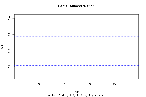
Title produced by software

(Partial) Autocorrelation Function

Date of computation

Sun, 19 Dec 2010 12:30:15 +0000

Cite this page as follows

Statistical Computations at FreeStatistics.org, Office for Research Development and Education, URL https://freestatistics.org/blog/index.php?v=date/2010/Dec/19/t12927616905cr4uzzyg0fgdse.htm/, Retrieved Sat, 04 May 2024 23:36:41 +0000

Statistical Computations at FreeStatistics.org, Office for Research Development and Education, URL https://freestatistics.org/blog/index.php?pk=112322, Retrieved Sat, 04 May 2024 23:36:41 +0000

QR Codes:

Paste this QR Code to cite your computation.

Original text written by user:

IsPrivate?

No (this computation is public)

User-defined keywords

Estimated Impact

147

Family? (F = Feedback message, R = changed R code, M = changed R Module, P = changed Parameters, D = changed Data)

F     [Univariate Data Series] [HPC Retail Sales] [2008-03-02 15:42:48] [74be16979710d4c4e7c6647856088456]
-  MPD  [Univariate Data Series] [WS8 1] [2010-11-30 15:47:30] [07a238a5afc23eb944f8545182f29d5a]
- RMP     [Classical Decomposition] [WS8 2] [2010-11-30 15:54:02] [07a238a5afc23eb944f8545182f29d5a]
- RMPD      [Univariate Data Series] [Statistiek: Werkl...] [2010-12-12 15:20:09] [07a238a5afc23eb944f8545182f29d5a]
-    D        [Univariate Data Series] [Statistiek: Werkl...] [2010-12-14 09:08:05] [07a238a5afc23eb944f8545182f29d5a]
-               [Univariate Data Series] [Statistiek: Werkl...] [2010-12-14 09:12:36] [07a238a5afc23eb944f8545182f29d5a]
- RMPD            [Classical Decomposition] [statistiek classi...] [2010-12-19 09:09:14] [07a238a5afc23eb944f8545182f29d5a]
- RMP               [(Partial) Autocorrelation Function] [Statistiek: ACF D...] [2010-12-19 10:44:26] [07a238a5afc23eb944f8545182f29d5a]
-   P                   [(Partial) Autocorrelation Function] [Statistiek: ACF D...] [2010-12-19 12:30:15] [67e3c2d70de1dbb070b545ca6c893d5e] [Current]
-   P                     [(Partial) Autocorrelation Function] [Statistiek: ACF D...] [2010-12-19 12:34:49] [07a238a5afc23eb944f8545182f29d5a] 
-   P                       [(Partial) Autocorrelation Function] [Statistiek: ACF D...] [2010-12-19 12:39:46] [07a238a5afc23eb944f8545182f29d5a] 
- RM                          [Spectral Analysis] [statistiek: spectrum] [2010-12-19 12:54:11] [07a238a5afc23eb944f8545182f29d5a] 
- RM                            [Variance Reduction Matrix] [statistiek: VRM] [2010-12-19 12:56:08] [07a238a5afc23eb944f8545182f29d5a] 
- RMP                           [(Partial) Autocorrelation Function] [statistiek: spect...] [2010-12-19 19:42:47] [07a238a5afc23eb944f8545182f29d5a] 
-   P                           [Spectral Analysis] [statistiek: spect...] [2010-12-19 19:43:57] [07a238a5afc23eb944f8545182f29d5a] 
-   P                           [Spectral Analysis] [statistiek: spect...] [2010-12-20 19:00:08] [07a238a5afc23eb944f8545182f29d5a] 
-   P                         [(Partial) Autocorrelation Function] [statistiek: ACF M...] [2010-12-19 19:53:24] [07a238a5afc23eb944f8545182f29d5a] 
- RMP                       [Standard Deviation-Mean Plot] [statistiek: stada...] [2010-12-19 15:02:29] [07a238a5afc23eb944f8545182f29d5a] 
- RMP                         [ARIMA Backward Selection] [Statistiek: Arima...] [2010-12-20 19:29:57] [07a238a5afc23eb944f8545182f29d5a] 
- RMP                           [ARIMA Forecasting] [statistiek: Arima...] [2010-12-20 19:46:41] [07a238a5afc23eb944f8545182f29d5a] 

Feedback Forum

Post a new message

Dataseries X:

Download CSV

Histogram

Boxplots

6.5
6.3
5.9
5.5
5.2
4.9
5.4
5.8
5.7
5.6
5.5
5.4
5.4
5.4
5.5
5.8
5.7
5.4
5.6
5.8
6.2
6.8
6.7
6.7
6.4
6.3
6.3
6.4
6.3
6
6.3
6.3
6.6
7.5
7.8
7.9
7.8
7.6
7.5
7.6
7.5
7.3
7.6
7.5
7.6
7.9
7.9
8.1
8.2
8
7.5
6.8
6.5
6.6
7.6
8
8.1
7.7
7.5
7.6
7.8
7.8
7.8
7.5
7.5
7.1
7.5
7.5
7.6
7.7
7.7
7.9
8.1
8.2
8.2
8.2
7.9
7.3
6.9
6.6
6.7
6.9
7
7.1
7.2
7.1
6.9
7
6.8
6.4
6.7
6.6
6.4
6.3
6.2
6.5
6.8
6.8
6.4
6.1
5.8
6.1
7.2
7.3
6.9
6.1
5.8
6.2
7.1
7.7
8
7.8
7.4
7.4
7.7
7.8
7.8
8
8.1
8.4

Summary of computational transaction
Raw Input	view raw input (R code)
Raw Output	view raw output of R engine
Computing time	2 seconds
R Server	'RServer@AstonUniversity' @ vre.aston.ac.uk

\begin{tabular}{lllllllll}
\hline
Summary of computational transaction \tabularnewline
Raw Input & view raw input (R code)  \tabularnewline
Raw Output & view raw output of R engine  \tabularnewline
Computing time & 2 seconds \tabularnewline
R Server & 'RServer@AstonUniversity' @ vre.aston.ac.uk \tabularnewline
\hline
\end{tabular}
%Source: https://freestatistics.org/blog/index.php?pk=112322&T=0

[TABLE]
[ROW][C]Summary of computational transaction[/C][/ROW]
[ROW][C]Raw Input[/C][C]view raw input (R code) [/C][/ROW]
[ROW][C]Raw Output[/C][C]view raw output of R engine [/C][/ROW]
[ROW][C]Computing time[/C][C]2 seconds[/C][/ROW]
[ROW][C]R Server[/C][C]'RServer@AstonUniversity' @ vre.aston.ac.uk[/C][/ROW]
[/TABLE]
Source: https://freestatistics.org/blog/index.php?pk=112322&T=0

Globally Unique Identifier (entire table): ba.freestatistics.org/blog/index.php?pk=112322&T=0

As an alternative you can also use a QR Code:

The GUIDs for individual cells are displayed in the table below:

Summary of computational transaction
Raw Input	view raw input (R code)
Raw Output	view raw output of R engine
Computing time	2 seconds
R Server	'RServer@AstonUniversity' @ vre.aston.ac.uk

Autocorrelation Function
Time lag k	ACF(k)	T-STAT	P-value
1	0.420361	4.5856	6e-06
2	-0.084225	-0.9188	0.180033
3	-0.408441	-4.4556	1e-05
4	-0.431285	-4.7048	3e-06
5	-0.066113	-0.7212	0.236098
6	0.240583	2.6244	0.004908
7	0.19541	2.1317	0.017545
8	-0.021227	-0.2316	0.408638
9	-0.129623	-1.414	0.079984
10	-0.18835	-2.0547	0.021051
11	-0.017438	-0.1902	0.424728
12	0.314308	3.4287	0.000417
13	0.145378	1.5859	0.05771
14	0.136785	1.4922	0.069153
15	0.059687	0.6511	0.258115
16	-0.151966	-1.6578	0.05
17	-0.16222	-1.7696	0.039677
18	-0.143075	-1.5608	0.060618
19	-0.063527	-0.693	0.244831
20	0.01549	0.169	0.43305
21	0.11969	1.3057	0.097092
22	-0.00309	-0.0337	0.486582
23	-0.106935	-1.1665	0.122868
24	-0.023897	-0.2607	0.397392

\begin{tabular}{lllllllll}
\hline
Autocorrelation Function \tabularnewline
Time lag k & ACF(k) & T-STAT & P-value \tabularnewline
1 & 0.420361 & 4.5856 & 6e-06 \tabularnewline
2 & -0.084225 & -0.9188 & 0.180033 \tabularnewline
3 & -0.408441 & -4.4556 & 1e-05 \tabularnewline
4 & -0.431285 & -4.7048 & 3e-06 \tabularnewline
5 & -0.066113 & -0.7212 & 0.236098 \tabularnewline
6 & 0.240583 & 2.6244 & 0.004908 \tabularnewline
7 & 0.19541 & 2.1317 & 0.017545 \tabularnewline
8 & -0.021227 & -0.2316 & 0.408638 \tabularnewline
9 & -0.129623 & -1.414 & 0.079984 \tabularnewline
10 & -0.18835 & -2.0547 & 0.021051 \tabularnewline
11 & -0.017438 & -0.1902 & 0.424728 \tabularnewline
12 & 0.314308 & 3.4287 & 0.000417 \tabularnewline
13 & 0.145378 & 1.5859 & 0.05771 \tabularnewline
14 & 0.136785 & 1.4922 & 0.069153 \tabularnewline
15 & 0.059687 & 0.6511 & 0.258115 \tabularnewline
16 & -0.151966 & -1.6578 & 0.05 \tabularnewline
17 & -0.16222 & -1.7696 & 0.039677 \tabularnewline
18 & -0.143075 & -1.5608 & 0.060618 \tabularnewline
19 & -0.063527 & -0.693 & 0.244831 \tabularnewline
20 & 0.01549 & 0.169 & 0.43305 \tabularnewline
21 & 0.11969 & 1.3057 & 0.097092 \tabularnewline
22 & -0.00309 & -0.0337 & 0.486582 \tabularnewline
23 & -0.106935 & -1.1665 & 0.122868 \tabularnewline
24 & -0.023897 & -0.2607 & 0.397392 \tabularnewline
\hline
\end{tabular}
%Source: https://freestatistics.org/blog/index.php?pk=112322&T=1

[TABLE]
[ROW][C]Autocorrelation Function[/C][/ROW]
[ROW][C]Time lag k[/C][C]ACF(k)[/C][C]T-STAT[/C][C]P-value[/C][/ROW]
[ROW][C]1[/C][C]0.420361[/C][C]4.5856[/C][C]6e-06[/C][/ROW]
[ROW][C]2[/C][C]-0.084225[/C][C]-0.9188[/C][C]0.180033[/C][/ROW]
[ROW][C]3[/C][C]-0.408441[/C][C]-4.4556[/C][C]1e-05[/C][/ROW]
[ROW][C]4[/C][C]-0.431285[/C][C]-4.7048[/C][C]3e-06[/C][/ROW]
[ROW][C]5[/C][C]-0.066113[/C][C]-0.7212[/C][C]0.236098[/C][/ROW]
[ROW][C]6[/C][C]0.240583[/C][C]2.6244[/C][C]0.004908[/C][/ROW]
[ROW][C]7[/C][C]0.19541[/C][C]2.1317[/C][C]0.017545[/C][/ROW]
[ROW][C]8[/C][C]-0.021227[/C][C]-0.2316[/C][C]0.408638[/C][/ROW]
[ROW][C]9[/C][C]-0.129623[/C][C]-1.414[/C][C]0.079984[/C][/ROW]
[ROW][C]10[/C][C]-0.18835[/C][C]-2.0547[/C][C]0.021051[/C][/ROW]
[ROW][C]11[/C][C]-0.017438[/C][C]-0.1902[/C][C]0.424728[/C][/ROW]
[ROW][C]12[/C][C]0.314308[/C][C]3.4287[/C][C]0.000417[/C][/ROW]
[ROW][C]13[/C][C]0.145378[/C][C]1.5859[/C][C]0.05771[/C][/ROW]
[ROW][C]14[/C][C]0.136785[/C][C]1.4922[/C][C]0.069153[/C][/ROW]
[ROW][C]15[/C][C]0.059687[/C][C]0.6511[/C][C]0.258115[/C][/ROW]
[ROW][C]16[/C][C]-0.151966[/C][C]-1.6578[/C][C]0.05[/C][/ROW]
[ROW][C]17[/C][C]-0.16222[/C][C]-1.7696[/C][C]0.039677[/C][/ROW]
[ROW][C]18[/C][C]-0.143075[/C][C]-1.5608[/C][C]0.060618[/C][/ROW]
[ROW][C]19[/C][C]-0.063527[/C][C]-0.693[/C][C]0.244831[/C][/ROW]
[ROW][C]20[/C][C]0.01549[/C][C]0.169[/C][C]0.43305[/C][/ROW]
[ROW][C]21[/C][C]0.11969[/C][C]1.3057[/C][C]0.097092[/C][/ROW]
[ROW][C]22[/C][C]-0.00309[/C][C]-0.0337[/C][C]0.486582[/C][/ROW]
[ROW][C]23[/C][C]-0.106935[/C][C]-1.1665[/C][C]0.122868[/C][/ROW]
[ROW][C]24[/C][C]-0.023897[/C][C]-0.2607[/C][C]0.397392[/C][/ROW]
[/TABLE]
Source: https://freestatistics.org/blog/index.php?pk=112322&T=1

Globally Unique Identifier (entire table): ba.freestatistics.org/blog/index.php?pk=112322&T=1

As an alternative you can also use a QR Code:

The GUIDs for individual cells are displayed in the table below:

Autocorrelation Function
Time lag k	ACF(k)	T-STAT	P-value
1	0.420361	4.5856	6e-06
2	-0.084225	-0.9188	0.180033
3	-0.408441	-4.4556	1e-05
4	-0.431285	-4.7048	3e-06
5	-0.066113	-0.7212	0.236098
6	0.240583	2.6244	0.004908
7	0.19541	2.1317	0.017545
8	-0.021227	-0.2316	0.408638
9	-0.129623	-1.414	0.079984
10	-0.18835	-2.0547	0.021051
11	-0.017438	-0.1902	0.424728
12	0.314308	3.4287	0.000417
13	0.145378	1.5859	0.05771
14	0.136785	1.4922	0.069153
15	0.059687	0.6511	0.258115
16	-0.151966	-1.6578	0.05
17	-0.16222	-1.7696	0.039677
18	-0.143075	-1.5608	0.060618
19	-0.063527	-0.693	0.244831
20	0.01549	0.169	0.43305
21	0.11969	1.3057	0.097092
22	-0.00309	-0.0337	0.486582
23	-0.106935	-1.1665	0.122868
24	-0.023897	-0.2607	0.397392

Partial Autocorrelation Function
Time lag k	PACF(k)	T-STAT	P-value
1	0.420361	4.5856	6e-06
2	-0.316931	-3.4573	0.000379
3	-0.308654	-3.367	0.000512
4	-0.190568	-2.0788	0.01989
5	0.147871	1.6131	0.054688
6	0.070602	0.7702	0.221362
7	-0.172827	-1.8853	0.030913
8	-0.143282	-1.563	0.060351
9	0.093422	1.0191	0.155108
10	-0.074524	-0.813	0.208933
11	0.005928	0.0647	0.474275
12	0.296851	3.2383	0.000779
13	-0.237983	-2.5961	0.005308
14	0.285655	3.1161	0.001149
15	0.193987	2.1162	0.018208
16	-0.159454	-1.7394	0.042272
17	-0.058477	-0.6379	0.262378
18	-0.043857	-0.4784	0.316614
19	0.085095	0.9283	0.177572
20	-0.130426	-1.4228	0.078708
21	-0.031038	-0.3386	0.367758
22	-0.063457	-0.6922	0.245071
23	-0.164799	-1.7977	0.037376
24	0.04312	0.4704	0.31947

\begin{tabular}{lllllllll}
\hline
Partial Autocorrelation Function \tabularnewline
Time lag k & PACF(k) & T-STAT & P-value \tabularnewline
1 & 0.420361 & 4.5856 & 6e-06 \tabularnewline
2 & -0.316931 & -3.4573 & 0.000379 \tabularnewline
3 & -0.308654 & -3.367 & 0.000512 \tabularnewline
4 & -0.190568 & -2.0788 & 0.01989 \tabularnewline
5 & 0.147871 & 1.6131 & 0.054688 \tabularnewline
6 & 0.070602 & 0.7702 & 0.221362 \tabularnewline
7 & -0.172827 & -1.8853 & 0.030913 \tabularnewline
8 & -0.143282 & -1.563 & 0.060351 \tabularnewline
9 & 0.093422 & 1.0191 & 0.155108 \tabularnewline
10 & -0.074524 & -0.813 & 0.208933 \tabularnewline
11 & 0.005928 & 0.0647 & 0.474275 \tabularnewline
12 & 0.296851 & 3.2383 & 0.000779 \tabularnewline
13 & -0.237983 & -2.5961 & 0.005308 \tabularnewline
14 & 0.285655 & 3.1161 & 0.001149 \tabularnewline
15 & 0.193987 & 2.1162 & 0.018208 \tabularnewline
16 & -0.159454 & -1.7394 & 0.042272 \tabularnewline
17 & -0.058477 & -0.6379 & 0.262378 \tabularnewline
18 & -0.043857 & -0.4784 & 0.316614 \tabularnewline
19 & 0.085095 & 0.9283 & 0.177572 \tabularnewline
20 & -0.130426 & -1.4228 & 0.078708 \tabularnewline
21 & -0.031038 & -0.3386 & 0.367758 \tabularnewline
22 & -0.063457 & -0.6922 & 0.245071 \tabularnewline
23 & -0.164799 & -1.7977 & 0.037376 \tabularnewline
24 & 0.04312 & 0.4704 & 0.31947 \tabularnewline
\hline
\end{tabular}
%Source: https://freestatistics.org/blog/index.php?pk=112322&T=2

[TABLE]
[ROW][C]Partial Autocorrelation Function[/C][/ROW]
[ROW][C]Time lag k[/C][C]PACF(k)[/C][C]T-STAT[/C][C]P-value[/C][/ROW]
[ROW][C]1[/C][C]0.420361[/C][C]4.5856[/C][C]6e-06[/C][/ROW]
[ROW][C]2[/C][C]-0.316931[/C][C]-3.4573[/C][C]0.000379[/C][/ROW]
[ROW][C]3[/C][C]-0.308654[/C][C]-3.367[/C][C]0.000512[/C][/ROW]
[ROW][C]4[/C][C]-0.190568[/C][C]-2.0788[/C][C]0.01989[/C][/ROW]
[ROW][C]5[/C][C]0.147871[/C][C]1.6131[/C][C]0.054688[/C][/ROW]
[ROW][C]6[/C][C]0.070602[/C][C]0.7702[/C][C]0.221362[/C][/ROW]
[ROW][C]7[/C][C]-0.172827[/C][C]-1.8853[/C][C]0.030913[/C][/ROW]
[ROW][C]8[/C][C]-0.143282[/C][C]-1.563[/C][C]0.060351[/C][/ROW]
[ROW][C]9[/C][C]0.093422[/C][C]1.0191[/C][C]0.155108[/C][/ROW]
[ROW][C]10[/C][C]-0.074524[/C][C]-0.813[/C][C]0.208933[/C][/ROW]
[ROW][C]11[/C][C]0.005928[/C][C]0.0647[/C][C]0.474275[/C][/ROW]
[ROW][C]12[/C][C]0.296851[/C][C]3.2383[/C][C]0.000779[/C][/ROW]
[ROW][C]13[/C][C]-0.237983[/C][C]-2.5961[/C][C]0.005308[/C][/ROW]
[ROW][C]14[/C][C]0.285655[/C][C]3.1161[/C][C]0.001149[/C][/ROW]
[ROW][C]15[/C][C]0.193987[/C][C]2.1162[/C][C]0.018208[/C][/ROW]
[ROW][C]16[/C][C]-0.159454[/C][C]-1.7394[/C][C]0.042272[/C][/ROW]
[ROW][C]17[/C][C]-0.058477[/C][C]-0.6379[/C][C]0.262378[/C][/ROW]
[ROW][C]18[/C][C]-0.043857[/C][C]-0.4784[/C][C]0.316614[/C][/ROW]
[ROW][C]19[/C][C]0.085095[/C][C]0.9283[/C][C]0.177572[/C][/ROW]
[ROW][C]20[/C][C]-0.130426[/C][C]-1.4228[/C][C]0.078708[/C][/ROW]
[ROW][C]21[/C][C]-0.031038[/C][C]-0.3386[/C][C]0.367758[/C][/ROW]
[ROW][C]22[/C][C]-0.063457[/C][C]-0.6922[/C][C]0.245071[/C][/ROW]
[ROW][C]23[/C][C]-0.164799[/C][C]-1.7977[/C][C]0.037376[/C][/ROW]
[ROW][C]24[/C][C]0.04312[/C][C]0.4704[/C][C]0.31947[/C][/ROW]
[/TABLE]
Source: https://freestatistics.org/blog/index.php?pk=112322&T=2

Globally Unique Identifier (entire table): ba.freestatistics.org/blog/index.php?pk=112322&T=2

As an alternative you can also use a QR Code:

The GUIDs for individual cells are displayed in the table below:

Partial Autocorrelation Function
Time lag k	PACF(k)	T-STAT	P-value
1	0.420361	4.5856	6e-06
2	-0.316931	-3.4573	0.000379
3	-0.308654	-3.367	0.000512
4	-0.190568	-2.0788	0.01989
5	0.147871	1.6131	0.054688
6	0.070602	0.7702	0.221362
7	-0.172827	-1.8853	0.030913
8	-0.143282	-1.563	0.060351
9	0.093422	1.0191	0.155108
10	-0.074524	-0.813	0.208933
11	0.005928	0.0647	0.474275
12	0.296851	3.2383	0.000779
13	-0.237983	-2.5961	0.005308
14	0.285655	3.1161	0.001149
15	0.193987	2.1162	0.018208
16	-0.159454	-1.7394	0.042272
17	-0.058477	-0.6379	0.262378
18	-0.043857	-0.4784	0.316614
19	0.085095	0.9283	0.177572
20	-0.130426	-1.4228	0.078708
21	-0.031038	-0.3386	0.367758
22	-0.063457	-0.6922	0.245071
23	-0.164799	-1.7977	0.037376
24	0.04312	0.4704	0.31947

Figure 1

PNG link

Postscript link

PDF link

Figure 2

PNG link

Postscript link

PDF link

Figure 3

PNG link

Postscript link

PDF link

Parameters (Session):

par1 = 24 ; par2 = 1 ; par3 = 1 ; par4 = 0 ; par5 = 12 ; par6 = White Noise ; par7 = 0.95 ;

Parameters (R input):

par1 = 24 ; par2 = 1 ; par3 = 1 ; par4 = 0 ; par5 = 12 ; par6 = White Noise ; par7 = 0.95 ; par8 = ;

R code (references can be found in the software module):

if (par1 == 'Default') {
par1 = 10*log10(length(x))
} else {
par1 <- as.numeric(par1)
}
par2 <- as.numeric(par2)
par3 <- as.numeric(par3)
par4 <- as.numeric(par4)
par5 <- as.numeric(par5)
if (par6 == 'White Noise') par6 <- 'white' else par6 <- 'ma'
par7 <- as.numeric(par7)
if (par8 != '') par8 <- as.numeric(par8)
ox <- x
if (par8 == '') {
if (par2 == 0) {
x <- log(x)
} else {
x <- (x ^ par2 - 1) / par2
}
} else {
x <- log(x,base=par8)
}
if (par3 > 0) x <- diff(x,lag=1,difference=par3)
if (par4 > 0) x <- diff(x,lag=par5,difference=par4)
bitmap(file='picts.png')
op <- par(mfrow=c(2,1))
plot(ox,type='l',main='Original Time Series',xlab='time',ylab='value')
if (par8=='') {
mytitle <- paste('Working Time Series (lambda=',par2,', d=',par3,', D=',par4,')',sep='')
mysub <- paste('(lambda=',par2,', d=',par3,', D=',par4,', CI=', par7, ', CI type=',par6,')',sep='')
} else {
mytitle <- paste('Working Time Series (base=',par8,', d=',par3,', D=',par4,')',sep='')
mysub <- paste('(base=',par8,', d=',par3,', D=',par4,', CI=', par7, ', CI type=',par6,')',sep='')
}
plot(x,type='l', main=mytitle,xlab='time',ylab='value')
par(op)
dev.off()
bitmap(file='pic1.png')
racf <- acf(x, par1, main='Autocorrelation', xlab='time lag', ylab='ACF', ci.type=par6, ci=par7, sub=mysub)
dev.off()
bitmap(file='pic2.png')
rpacf <- pacf(x,par1,main='Partial Autocorrelation',xlab='lags',ylab='PACF',sub=mysub)
dev.off()
(myacf <- c(racf$acf))
(mypacf <- c(rpacf$acf))
lengthx <- length(x)
sqrtn <- sqrt(lengthx)
load(file='createtable')
a<-table.start()
a<-table.row.start(a)
a<-table.element(a,'Autocorrelation Function',4,TRUE)
a<-table.row.end(a)
a<-table.row.start(a)
a<-table.element(a,'Time lag k',header=TRUE)
a<-table.element(a,hyperlink('basics.htm','ACF(k)','click here for more information about the Autocorrelation Function'),header=TRUE)
a<-table.element(a,'T-STAT',header=TRUE)
a<-table.element(a,'P-value',header=TRUE)
a<-table.row.end(a)
for (i in 2:(par1+1)) {
a<-table.row.start(a)
a<-table.element(a,i-1,header=TRUE)
a<-table.element(a,round(myacf[i],6))
mytstat <- myacf[i]*sqrtn
a<-table.element(a,round(mytstat,4))
a<-table.element(a,round(1-pt(abs(mytstat),lengthx),6))
a<-table.row.end(a)
}
a<-table.end(a)
table.save(a,file='mytable.tab')
a<-table.start()
a<-table.row.start(a)
a<-table.element(a,'Partial Autocorrelation Function',4,TRUE)
a<-table.row.end(a)
a<-table.row.start(a)
a<-table.element(a,'Time lag k',header=TRUE)
a<-table.element(a,hyperlink('basics.htm','PACF(k)','click here for more information about the Partial Autocorrelation Function'),header=TRUE)
a<-table.element(a,'T-STAT',header=TRUE)
a<-table.element(a,'P-value',header=TRUE)
a<-table.row.end(a)
for (i in 1:par1) {
a<-table.row.start(a)
a<-table.element(a,i,header=TRUE)
a<-table.element(a,round(mypacf[i],6))
mytstat <- mypacf[i]*sqrtn
a<-table.element(a,round(mytstat,4))
a<-table.element(a,round(1-pt(abs(mytstat),lengthx),6))
a<-table.row.end(a)
}
a<-table.end(a)
table.save(a,file='mytable1.tab')

Free Statistics

Description of Statistical Computation

Tree of Dependent Computations

Dataset

Tables (Output of Computation)

Figures (Output of Computation)

Input Parameters & R Code