Repository of Reproducible Computations

Free Statistics

of Irreproducible Research!

Author's title

Author

*The author of this computation has been verified*

R Software Module

rwasp_autocorrelation.wasp

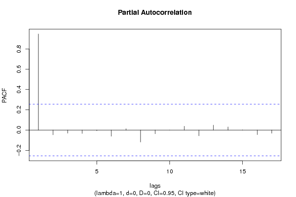
Title produced by software

(Partial) Autocorrelation Function

Date of computation

Sat, 18 Dec 2010 17:47:34 +0000

Cite this page as follows

Statistical Computations at FreeStatistics.org, Office for Research Development and Education, URL https://freestatistics.org/blog/index.php?v=date/2010/Dec/18/t12926943482iy9bohbuj0jw1b.htm/, Retrieved Tue, 30 Apr 2024 07:53:12 +0000

Statistical Computations at FreeStatistics.org, Office for Research Development and Education, URL https://freestatistics.org/blog/index.php?pk=112133, Retrieved Tue, 30 Apr 2024 07:53:12 +0000

QR Codes:

Paste this QR Code to cite your computation.

Original text written by user:

IsPrivate?

No (this computation is public)

User-defined keywords

Estimated Impact

176

Family? (F = Feedback message, R = changed R code, M = changed R Module, P = changed Parameters, D = changed Data)

-     [Multiple Regression] [Q1 The Seatbeltlaw] [2007-11-14 19:27:43] [8cd6641b921d30ebe00b648d1481bba0]
- RMPD  [Multiple Regression] [Seatbelt] [2009-11-12 13:54:52] [b98453cac15ba1066b407e146608df68]
- R  D    [Multiple Regression] [Paper TSA Multipl...] [2010-12-18 12:51:38] [945bcebba5e7ac34a41d6888338a1ba9]
-   P       [Multiple Regression] [Paper TSA Multipl...] [2010-12-18 13:26:55] [945bcebba5e7ac34a41d6888338a1ba9]
-    D        [Multiple Regression] [Paper TSA Multipl...] [2010-12-18 15:54:00] [945bcebba5e7ac34a41d6888338a1ba9]
- RMPD            [(Partial) Autocorrelation Function] [Paper TSA ACF] [2010-12-18 17:47:34] [514029464b0621595fe21c9fa38c7009] [Current]

Feedback Forum

Post a new message

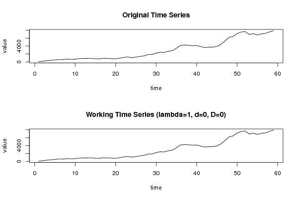
Dataseries X:

Download CSV

Histogram

Boxplots

Summary of computational transaction
Raw Input	view raw input (R code)
Raw Output	view raw output of R engine
Computing time	2 seconds
R Server	'Gwilym Jenkins' @ 72.249.127.135

\begin{tabular}{lllllllll}
\hline
Summary of computational transaction \tabularnewline
Raw Input & view raw input (R code)  \tabularnewline
Raw Output & view raw output of R engine  \tabularnewline
Computing time & 2 seconds \tabularnewline
R Server & 'Gwilym Jenkins' @ 72.249.127.135 \tabularnewline
\hline
\end{tabular}
%Source: https://freestatistics.org/blog/index.php?pk=112133&T=0

[TABLE]
[ROW][C]Summary of computational transaction[/C][/ROW]
[ROW][C]Raw Input[/C][C]view raw input (R code) [/C][/ROW]
[ROW][C]Raw Output[/C][C]view raw output of R engine [/C][/ROW]
[ROW][C]Computing time[/C][C]2 seconds[/C][/ROW]
[ROW][C]R Server[/C][C]'Gwilym Jenkins' @ 72.249.127.135[/C][/ROW]
[/TABLE]
Source: https://freestatistics.org/blog/index.php?pk=112133&T=0

Globally Unique Identifier (entire table): ba.freestatistics.org/blog/index.php?pk=112133&T=0

As an alternative you can also use a QR Code:

The GUIDs for individual cells are displayed in the table below:

Summary of computational transaction
Raw Input	view raw input (R code)
Raw Output	view raw output of R engine
Computing time	2 seconds
R Server	'Gwilym Jenkins' @ 72.249.127.135

Autocorrelation Function
Time lag k	ACF(k)	T-STAT	P-value
1	0.947347	7.2767	0
2	0.892633	6.8564	0
3	0.837716	6.4346	0
4	0.782399	6.0097	0
5	0.729564	5.6039	0
6	0.673674	5.1746	1e-06
7	0.622432	4.781	6e-06
8	0.562564	4.3211	3e-05
9	0.502412	3.8591	0.000142
10	0.446485	3.4295	0.000555
11	0.39801	3.0572	0.001677
12	0.348377	2.6759	0.004816
13	0.306543	2.3546	0.010945
14	0.27217	2.0906	0.020441
15	0.240366	1.8463	0.034934
16	0.207271	1.5921	0.058355
17	0.17349	1.3326	0.093893

\begin{tabular}{lllllllll}
\hline
Autocorrelation Function \tabularnewline
Time lag k & ACF(k) & T-STAT & P-value \tabularnewline
1 & 0.947347 & 7.2767 & 0 \tabularnewline
2 & 0.892633 & 6.8564 & 0 \tabularnewline
3 & 0.837716 & 6.4346 & 0 \tabularnewline
4 & 0.782399 & 6.0097 & 0 \tabularnewline
5 & 0.729564 & 5.6039 & 0 \tabularnewline
6 & 0.673674 & 5.1746 & 1e-06 \tabularnewline
7 & 0.622432 & 4.781 & 6e-06 \tabularnewline
8 & 0.562564 & 4.3211 & 3e-05 \tabularnewline
9 & 0.502412 & 3.8591 & 0.000142 \tabularnewline
10 & 0.446485 & 3.4295 & 0.000555 \tabularnewline
11 & 0.39801 & 3.0572 & 0.001677 \tabularnewline
12 & 0.348377 & 2.6759 & 0.004816 \tabularnewline
13 & 0.306543 & 2.3546 & 0.010945 \tabularnewline
14 & 0.27217 & 2.0906 & 0.020441 \tabularnewline
15 & 0.240366 & 1.8463 & 0.034934 \tabularnewline
16 & 0.207271 & 1.5921 & 0.058355 \tabularnewline
17 & 0.17349 & 1.3326 & 0.093893 \tabularnewline
\hline
\end{tabular}
%Source: https://freestatistics.org/blog/index.php?pk=112133&T=1

[TABLE]
[ROW][C]Autocorrelation Function[/C][/ROW]
[ROW][C]Time lag k[/C][C]ACF(k)[/C][C]T-STAT[/C][C]P-value[/C][/ROW]
[ROW][C]1[/C][C]0.947347[/C][C]7.2767[/C][C]0[/C][/ROW]
[ROW][C]2[/C][C]0.892633[/C][C]6.8564[/C][C]0[/C][/ROW]
[ROW][C]3[/C][C]0.837716[/C][C]6.4346[/C][C]0[/C][/ROW]
[ROW][C]4[/C][C]0.782399[/C][C]6.0097[/C][C]0[/C][/ROW]
[ROW][C]5[/C][C]0.729564[/C][C]5.6039[/C][C]0[/C][/ROW]
[ROW][C]6[/C][C]0.673674[/C][C]5.1746[/C][C]1e-06[/C][/ROW]
[ROW][C]7[/C][C]0.622432[/C][C]4.781[/C][C]6e-06[/C][/ROW]
[ROW][C]8[/C][C]0.562564[/C][C]4.3211[/C][C]3e-05[/C][/ROW]
[ROW][C]9[/C][C]0.502412[/C][C]3.8591[/C][C]0.000142[/C][/ROW]
[ROW][C]10[/C][C]0.446485[/C][C]3.4295[/C][C]0.000555[/C][/ROW]
[ROW][C]11[/C][C]0.39801[/C][C]3.0572[/C][C]0.001677[/C][/ROW]
[ROW][C]12[/C][C]0.348377[/C][C]2.6759[/C][C]0.004816[/C][/ROW]
[ROW][C]13[/C][C]0.306543[/C][C]2.3546[/C][C]0.010945[/C][/ROW]
[ROW][C]14[/C][C]0.27217[/C][C]2.0906[/C][C]0.020441[/C][/ROW]
[ROW][C]15[/C][C]0.240366[/C][C]1.8463[/C][C]0.034934[/C][/ROW]
[ROW][C]16[/C][C]0.207271[/C][C]1.5921[/C][C]0.058355[/C][/ROW]
[ROW][C]17[/C][C]0.17349[/C][C]1.3326[/C][C]0.093893[/C][/ROW]
[/TABLE]
Source: https://freestatistics.org/blog/index.php?pk=112133&T=1

Globally Unique Identifier (entire table): ba.freestatistics.org/blog/index.php?pk=112133&T=1

As an alternative you can also use a QR Code:

The GUIDs for individual cells are displayed in the table below:

Autocorrelation Function
Time lag k	ACF(k)	T-STAT	P-value
1	0.947347	7.2767	0
2	0.892633	6.8564	0
3	0.837716	6.4346	0
4	0.782399	6.0097	0
5	0.729564	5.6039	0
6	0.673674	5.1746	1e-06
7	0.622432	4.781	6e-06
8	0.562564	4.3211	3e-05
9	0.502412	3.8591	0.000142
10	0.446485	3.4295	0.000555
11	0.39801	3.0572	0.001677
12	0.348377	2.6759	0.004816
13	0.306543	2.3546	0.010945
14	0.27217	2.0906	0.020441
15	0.240366	1.8463	0.034934
16	0.207271	1.5921	0.058355
17	0.17349	1.3326	0.093893

Partial Autocorrelation Function
Time lag k	PACF(k)	T-STAT	P-value
1	0.947347	7.2767	0
2	-0.047138	-0.3621	0.359294
3	-0.030522	-0.2344	0.407725
4	-0.033735	-0.2591	0.39822
5	-0.006572	-0.0505	0.479956
6	-0.061392	-0.4716	0.319491
7	0.013386	0.1028	0.459227
8	-0.118421	-0.9096	0.183366
9	-0.03675	-0.2823	0.389359
10	-7e-06	-1e-04	0.499979
11	0.037811	0.2904	0.386253
12	-0.05677	-0.4361	0.332192
13	0.048495	0.3725	0.355428
14	0.031093	0.2388	0.406034
15	0.002033	0.0156	0.493797
16	-0.045622	-0.3504	0.363632
17	-0.031393	-0.2411	0.405143

\begin{tabular}{lllllllll}
\hline
Partial Autocorrelation Function \tabularnewline
Time lag k & PACF(k) & T-STAT & P-value \tabularnewline
1 & 0.947347 & 7.2767 & 0 \tabularnewline
2 & -0.047138 & -0.3621 & 0.359294 \tabularnewline
3 & -0.030522 & -0.2344 & 0.407725 \tabularnewline
4 & -0.033735 & -0.2591 & 0.39822 \tabularnewline
5 & -0.006572 & -0.0505 & 0.479956 \tabularnewline
6 & -0.061392 & -0.4716 & 0.319491 \tabularnewline
7 & 0.013386 & 0.1028 & 0.459227 \tabularnewline
8 & -0.118421 & -0.9096 & 0.183366 \tabularnewline
9 & -0.03675 & -0.2823 & 0.389359 \tabularnewline
10 & -7e-06 & -1e-04 & 0.499979 \tabularnewline
11 & 0.037811 & 0.2904 & 0.386253 \tabularnewline
12 & -0.05677 & -0.4361 & 0.332192 \tabularnewline
13 & 0.048495 & 0.3725 & 0.355428 \tabularnewline
14 & 0.031093 & 0.2388 & 0.406034 \tabularnewline
15 & 0.002033 & 0.0156 & 0.493797 \tabularnewline
16 & -0.045622 & -0.3504 & 0.363632 \tabularnewline
17 & -0.031393 & -0.2411 & 0.405143 \tabularnewline
\hline
\end{tabular}
%Source: https://freestatistics.org/blog/index.php?pk=112133&T=2

[TABLE]
[ROW][C]Partial Autocorrelation Function[/C][/ROW]
[ROW][C]Time lag k[/C][C]PACF(k)[/C][C]T-STAT[/C][C]P-value[/C][/ROW]
[ROW][C]1[/C][C]0.947347[/C][C]7.2767[/C][C]0[/C][/ROW]
[ROW][C]2[/C][C]-0.047138[/C][C]-0.3621[/C][C]0.359294[/C][/ROW]
[ROW][C]3[/C][C]-0.030522[/C][C]-0.2344[/C][C]0.407725[/C][/ROW]
[ROW][C]4[/C][C]-0.033735[/C][C]-0.2591[/C][C]0.39822[/C][/ROW]
[ROW][C]5[/C][C]-0.006572[/C][C]-0.0505[/C][C]0.479956[/C][/ROW]
[ROW][C]6[/C][C]-0.061392[/C][C]-0.4716[/C][C]0.319491[/C][/ROW]
[ROW][C]7[/C][C]0.013386[/C][C]0.1028[/C][C]0.459227[/C][/ROW]
[ROW][C]8[/C][C]-0.118421[/C][C]-0.9096[/C][C]0.183366[/C][/ROW]
[ROW][C]9[/C][C]-0.03675[/C][C]-0.2823[/C][C]0.389359[/C][/ROW]
[ROW][C]10[/C][C]-7e-06[/C][C]-1e-04[/C][C]0.499979[/C][/ROW]
[ROW][C]11[/C][C]0.037811[/C][C]0.2904[/C][C]0.386253[/C][/ROW]
[ROW][C]12[/C][C]-0.05677[/C][C]-0.4361[/C][C]0.332192[/C][/ROW]
[ROW][C]13[/C][C]0.048495[/C][C]0.3725[/C][C]0.355428[/C][/ROW]
[ROW][C]14[/C][C]0.031093[/C][C]0.2388[/C][C]0.406034[/C][/ROW]
[ROW][C]15[/C][C]0.002033[/C][C]0.0156[/C][C]0.493797[/C][/ROW]
[ROW][C]16[/C][C]-0.045622[/C][C]-0.3504[/C][C]0.363632[/C][/ROW]
[ROW][C]17[/C][C]-0.031393[/C][C]-0.2411[/C][C]0.405143[/C][/ROW]
[/TABLE]
Source: https://freestatistics.org/blog/index.php?pk=112133&T=2

Globally Unique Identifier (entire table): ba.freestatistics.org/blog/index.php?pk=112133&T=2

As an alternative you can also use a QR Code:

The GUIDs for individual cells are displayed in the table below:

Partial Autocorrelation Function
Time lag k	PACF(k)	T-STAT	P-value
1	0.947347	7.2767	0
2	-0.047138	-0.3621	0.359294
3	-0.030522	-0.2344	0.407725
4	-0.033735	-0.2591	0.39822
5	-0.006572	-0.0505	0.479956
6	-0.061392	-0.4716	0.319491
7	0.013386	0.1028	0.459227
8	-0.118421	-0.9096	0.183366
9	-0.03675	-0.2823	0.389359
10	-7e-06	-1e-04	0.499979
11	0.037811	0.2904	0.386253
12	-0.05677	-0.4361	0.332192
13	0.048495	0.3725	0.355428
14	0.031093	0.2388	0.406034
15	0.002033	0.0156	0.493797
16	-0.045622	-0.3504	0.363632
17	-0.031393	-0.2411	0.405143

Figure 1

PNG link

Postscript link

PDF link

Figure 2

PNG link

Postscript link

PDF link

Figure 3

PNG link

Postscript link

PDF link

Parameters (Session):

par1 = Default ; par2 = 1 ; par3 = 0 ; par4 = 0 ; par5 = 1 ; par6 = White Noise ; par7 = 0.95 ;

Parameters (R input):

par1 = Default ; par2 = 1 ; par3 = 0 ; par4 = 0 ; par5 = 1 ; par6 = White Noise ; par7 = 0.95 ; par8 = ;

R code (references can be found in the software module):

if (par1 == 'Default') {
par1 = 10*log10(length(x))
} else {
par1 <- as.numeric(par1)
}
par2 <- as.numeric(par2)
par3 <- as.numeric(par3)
par4 <- as.numeric(par4)
par5 <- as.numeric(par5)
if (par6 == 'White Noise') par6 <- 'white' else par6 <- 'ma'
par7 <- as.numeric(par7)
if (par8 != '') par8 <- as.numeric(par8)
ox <- x
if (par8 == '') {
if (par2 == 0) {
x <- log(x)
} else {
x <- (x ^ par2 - 1) / par2
}
} else {
x <- log(x,base=par8)
}
if (par3 > 0) x <- diff(x,lag=1,difference=par3)
if (par4 > 0) x <- diff(x,lag=par5,difference=par4)
bitmap(file='picts.png')
op <- par(mfrow=c(2,1))
plot(ox,type='l',main='Original Time Series',xlab='time',ylab='value')
if (par8=='') {
mytitle <- paste('Working Time Series (lambda=',par2,', d=',par3,', D=',par4,')',sep='')
mysub <- paste('(lambda=',par2,', d=',par3,', D=',par4,', CI=', par7, ', CI type=',par6,')',sep='')
} else {
mytitle <- paste('Working Time Series (base=',par8,', d=',par3,', D=',par4,')',sep='')
mysub <- paste('(base=',par8,', d=',par3,', D=',par4,', CI=', par7, ', CI type=',par6,')',sep='')
}
plot(x,type='l', main=mytitle,xlab='time',ylab='value')
par(op)
dev.off()
bitmap(file='pic1.png')
racf <- acf(x, par1, main='Autocorrelation', xlab='time lag', ylab='ACF', ci.type=par6, ci=par7, sub=mysub)
dev.off()
bitmap(file='pic2.png')
rpacf <- pacf(x,par1,main='Partial Autocorrelation',xlab='lags',ylab='PACF',sub=mysub)
dev.off()
(myacf <- c(racf$acf))
(mypacf <- c(rpacf$acf))
lengthx <- length(x)
sqrtn <- sqrt(lengthx)
load(file='createtable')
a<-table.start()
a<-table.row.start(a)
a<-table.element(a,'Autocorrelation Function',4,TRUE)
a<-table.row.end(a)
a<-table.row.start(a)
a<-table.element(a,'Time lag k',header=TRUE)
a<-table.element(a,hyperlink('basics.htm','ACF(k)','click here for more information about the Autocorrelation Function'),header=TRUE)
a<-table.element(a,'T-STAT',header=TRUE)
a<-table.element(a,'P-value',header=TRUE)
a<-table.row.end(a)
for (i in 2:(par1+1)) {
a<-table.row.start(a)
a<-table.element(a,i-1,header=TRUE)
a<-table.element(a,round(myacf[i],6))
mytstat <- myacf[i]*sqrtn
a<-table.element(a,round(mytstat,4))
a<-table.element(a,round(1-pt(abs(mytstat),lengthx),6))
a<-table.row.end(a)
}
a<-table.end(a)
table.save(a,file='mytable.tab')
a<-table.start()
a<-table.row.start(a)
a<-table.element(a,'Partial Autocorrelation Function',4,TRUE)
a<-table.row.end(a)
a<-table.row.start(a)
a<-table.element(a,'Time lag k',header=TRUE)
a<-table.element(a,hyperlink('basics.htm','PACF(k)','click here for more information about the Partial Autocorrelation Function'),header=TRUE)
a<-table.element(a,'T-STAT',header=TRUE)
a<-table.element(a,'P-value',header=TRUE)
a<-table.row.end(a)
for (i in 1:par1) {
a<-table.row.start(a)
a<-table.element(a,i,header=TRUE)
a<-table.element(a,round(mypacf[i],6))
mytstat <- mypacf[i]*sqrtn
a<-table.element(a,round(mytstat,4))
a<-table.element(a,round(1-pt(abs(mytstat),lengthx),6))
a<-table.row.end(a)
}
a<-table.end(a)
table.save(a,file='mytable1.tab')

Free Statistics

Description of Statistical Computation

Tree of Dependent Computations

Dataset

Tables (Output of Computation)

Figures (Output of Computation)

Input Parameters & R Code