Repository of Reproducible Computations

Free Statistics

of Irreproducible Research!

Author's title

Author

*The author of this computation has been verified*

R Software Module

rwasp_autocorrelation.wasp

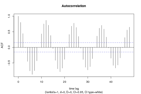
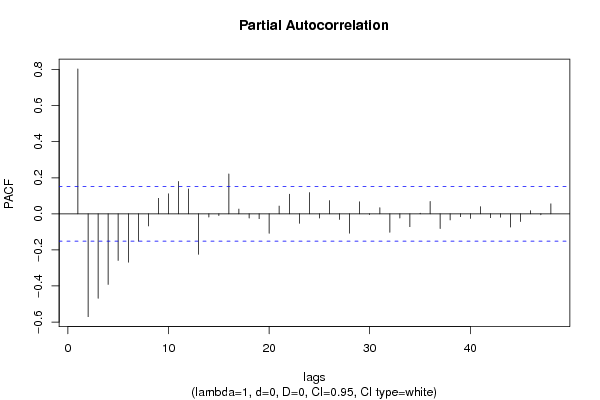
Title produced by software

(Partial) Autocorrelation Function

Date of computation

Sat, 18 Dec 2010 17:09:25 +0000

Cite this page as follows

Statistical Computations at FreeStatistics.org, Office for Research Development and Education, URL https://freestatistics.org/blog/index.php?v=date/2010/Dec/18/t12926932475nokddmw3dpbblw.htm/, Retrieved Tue, 30 Apr 2024 03:19:53 +0000

Statistical Computations at FreeStatistics.org, Office for Research Development and Education, URL https://freestatistics.org/blog/index.php?pk=112119, Retrieved Tue, 30 Apr 2024 03:19:53 +0000

QR Codes:

Paste this QR Code to cite your computation.

Original text written by user:

IsPrivate?

No (this computation is public)

User-defined keywords

Tom Aerts Julie Loockx

Estimated Impact

205

Family? (F = Feedback message, R = changed R code, M = changed R Module, P = changed Parameters, D = changed Data)

-       [(Partial) Autocorrelation Function] [Paper] [2010-12-18 17:09:25] [c2514e24605d0513c6bae17788e1fef3] [Current]
-   P     [(Partial) Autocorrelation Function] [Paper] [2010-12-22 10:04:19] [fa854ea294f510d944d2dbf77761bfce] 
-   PD    [(Partial) Autocorrelation Function] [acf] [2010-12-29 13:15:38] [e73e9643c012a54583c6a406017b2645] 
-   P       [(Partial) Autocorrelation Function] [ACF goed] [2010-12-29 13:27:42] [e73e9643c012a54583c6a406017b2645] 
-   P     [(Partial) Autocorrelation Function] [Paper ACF2] [2010-12-29 13:24:49] [fa854ea294f510d944d2dbf77761bfce] 
-   P     [(Partial) Autocorrelation Function] [Paper ] [2010-12-29 14:53:05] [fa854ea294f510d944d2dbf77761bfce] 

Feedback Forum

Post a new message

Dataseries X:

Download CSV

Histogram

Boxplots

Summary of computational transaction
Raw Input	view raw input (R code)
Raw Output	view raw output of R engine
Computing time	3 seconds
R Server	'George Udny Yule' @ 72.249.76.132

\begin{tabular}{lllllllll}
\hline
Summary of computational transaction \tabularnewline
Raw Input & view raw input (R code)  \tabularnewline
Raw Output & view raw output of R engine  \tabularnewline
Computing time & 3 seconds \tabularnewline
R Server & 'George Udny Yule' @ 72.249.76.132 \tabularnewline
\hline
\end{tabular}
%Source: https://freestatistics.org/blog/index.php?pk=112119&T=0

[TABLE]
[ROW][C]Summary of computational transaction[/C][/ROW]
[ROW][C]Raw Input[/C][C]view raw input (R code) [/C][/ROW]
[ROW][C]Raw Output[/C][C]view raw output of R engine [/C][/ROW]
[ROW][C]Computing time[/C][C]3 seconds[/C][/ROW]
[ROW][C]R Server[/C][C]'George Udny Yule' @ 72.249.76.132[/C][/ROW]
[/TABLE]
Source: https://freestatistics.org/blog/index.php?pk=112119&T=0

Globally Unique Identifier (entire table): ba.freestatistics.org/blog/index.php?pk=112119&T=0

As an alternative you can also use a QR Code:

The GUIDs for individual cells are displayed in the table below:

Summary of computational transaction
Raw Input	view raw input (R code)
Raw Output	view raw output of R engine
Computing time	3 seconds
R Server	'George Udny Yule' @ 72.249.76.132

Autocorrelation Function
Time lag k	ACF(k)	T-STAT	P-value
1	0.803317	10.4122	0
2	0.443069	5.7428	0
3	-0.011396	-0.1477	0.441375
4	-0.45167	-5.8543	0
5	-0.757133	-9.8136	0
6	-0.868159	-11.2526	0
7	-0.748508	-9.7018	0
8	-0.433509	-5.6189	0
9	0.001791	0.0232	0.490752
10	0.433734	5.6218	0
11	0.753782	9.7701	0
12	0.870128	11.2781	0
13	0.712437	9.2342	0
14	0.383594	4.9719	1e-06
15	-0.039253	-0.5088	0.305786
16	-0.417872	-5.4162	0
17	-0.689482	-8.9367	0
18	-0.784875	-10.1731	0
19	-0.668	-8.6583	0
20	-0.38585	-5.0012	1e-06
21	0.014363	0.1862	0.426272
22	0.41346	5.3591	0
23	0.681863	8.838	0
24	0.776447	10.0639	0
25	0.641142	8.3101	0
26	0.351356	4.5541	5e-06
27	-0.027047	-0.3506	0.363177
28	-0.389988	-5.0548	1e-06
29	-0.638776	-8.2795	0
30	-0.725397	-9.4022	0
31	-0.61967	-8.0318	0
32	-0.363228	-4.708	3e-06
33	0.005507	0.0714	0.47159
34	0.362332	4.6964	3e-06
35	0.616129	7.9859	0
36	0.709178	9.192	0
37	0.588139	7.6232	0
38	0.330991	4.2901	1.5e-05
39	-0.01634	-0.2118	0.416265
40	-0.350123	-4.5381	5e-06
41	-0.580392	-7.5227	0
42	-0.66365	-8.6019	0
43	-0.568291	-7.3659	0
44	-0.339387	-4.399	1e-05
45	-0.011167	-0.1447	0.442544
46	0.316942	4.108	3.1e-05
47	0.556793	7.2169	0
48	0.650699	8.434	0

\begin{tabular}{lllllllll}
\hline
Autocorrelation Function \tabularnewline
Time lag k & ACF(k) & T-STAT & P-value \tabularnewline
1 & 0.803317 & 10.4122 & 0 \tabularnewline
2 & 0.443069 & 5.7428 & 0 \tabularnewline
3 & -0.011396 & -0.1477 & 0.441375 \tabularnewline
4 & -0.45167 & -5.8543 & 0 \tabularnewline
5 & -0.757133 & -9.8136 & 0 \tabularnewline
6 & -0.868159 & -11.2526 & 0 \tabularnewline
7 & -0.748508 & -9.7018 & 0 \tabularnewline
8 & -0.433509 & -5.6189 & 0 \tabularnewline
9 & 0.001791 & 0.0232 & 0.490752 \tabularnewline
10 & 0.433734 & 5.6218 & 0 \tabularnewline
11 & 0.753782 & 9.7701 & 0 \tabularnewline
12 & 0.870128 & 11.2781 & 0 \tabularnewline
13 & 0.712437 & 9.2342 & 0 \tabularnewline
14 & 0.383594 & 4.9719 & 1e-06 \tabularnewline
15 & -0.039253 & -0.5088 & 0.305786 \tabularnewline
16 & -0.417872 & -5.4162 & 0 \tabularnewline
17 & -0.689482 & -8.9367 & 0 \tabularnewline
18 & -0.784875 & -10.1731 & 0 \tabularnewline
19 & -0.668 & -8.6583 & 0 \tabularnewline
20 & -0.38585 & -5.0012 & 1e-06 \tabularnewline
21 & 0.014363 & 0.1862 & 0.426272 \tabularnewline
22 & 0.41346 & 5.3591 & 0 \tabularnewline
23 & 0.681863 & 8.838 & 0 \tabularnewline
24 & 0.776447 & 10.0639 & 0 \tabularnewline
25 & 0.641142 & 8.3101 & 0 \tabularnewline
26 & 0.351356 & 4.5541 & 5e-06 \tabularnewline
27 & -0.027047 & -0.3506 & 0.363177 \tabularnewline
28 & -0.389988 & -5.0548 & 1e-06 \tabularnewline
29 & -0.638776 & -8.2795 & 0 \tabularnewline
30 & -0.725397 & -9.4022 & 0 \tabularnewline
31 & -0.61967 & -8.0318 & 0 \tabularnewline
32 & -0.363228 & -4.708 & 3e-06 \tabularnewline
33 & 0.005507 & 0.0714 & 0.47159 \tabularnewline
34 & 0.362332 & 4.6964 & 3e-06 \tabularnewline
35 & 0.616129 & 7.9859 & 0 \tabularnewline
36 & 0.709178 & 9.192 & 0 \tabularnewline
37 & 0.588139 & 7.6232 & 0 \tabularnewline
38 & 0.330991 & 4.2901 & 1.5e-05 \tabularnewline
39 & -0.01634 & -0.2118 & 0.416265 \tabularnewline
40 & -0.350123 & -4.5381 & 5e-06 \tabularnewline
41 & -0.580392 & -7.5227 & 0 \tabularnewline
42 & -0.66365 & -8.6019 & 0 \tabularnewline
43 & -0.568291 & -7.3659 & 0 \tabularnewline
44 & -0.339387 & -4.399 & 1e-05 \tabularnewline
45 & -0.011167 & -0.1447 & 0.442544 \tabularnewline
46 & 0.316942 & 4.108 & 3.1e-05 \tabularnewline
47 & 0.556793 & 7.2169 & 0 \tabularnewline
48 & 0.650699 & 8.434 & 0 \tabularnewline
\hline
\end{tabular}
%Source: https://freestatistics.org/blog/index.php?pk=112119&T=1

[TABLE]
[ROW][C]Autocorrelation Function[/C][/ROW]
[ROW][C]Time lag k[/C][C]ACF(k)[/C][C]T-STAT[/C][C]P-value[/C][/ROW]
[ROW][C]1[/C][C]0.803317[/C][C]10.4122[/C][C]0[/C][/ROW]
[ROW][C]2[/C][C]0.443069[/C][C]5.7428[/C][C]0[/C][/ROW]
[ROW][C]3[/C][C]-0.011396[/C][C]-0.1477[/C][C]0.441375[/C][/ROW]
[ROW][C]4[/C][C]-0.45167[/C][C]-5.8543[/C][C]0[/C][/ROW]
[ROW][C]5[/C][C]-0.757133[/C][C]-9.8136[/C][C]0[/C][/ROW]
[ROW][C]6[/C][C]-0.868159[/C][C]-11.2526[/C][C]0[/C][/ROW]
[ROW][C]7[/C][C]-0.748508[/C][C]-9.7018[/C][C]0[/C][/ROW]
[ROW][C]8[/C][C]-0.433509[/C][C]-5.6189[/C][C]0[/C][/ROW]
[ROW][C]9[/C][C]0.001791[/C][C]0.0232[/C][C]0.490752[/C][/ROW]
[ROW][C]10[/C][C]0.433734[/C][C]5.6218[/C][C]0[/C][/ROW]
[ROW][C]11[/C][C]0.753782[/C][C]9.7701[/C][C]0[/C][/ROW]
[ROW][C]12[/C][C]0.870128[/C][C]11.2781[/C][C]0[/C][/ROW]
[ROW][C]13[/C][C]0.712437[/C][C]9.2342[/C][C]0[/C][/ROW]
[ROW][C]14[/C][C]0.383594[/C][C]4.9719[/C][C]1e-06[/C][/ROW]
[ROW][C]15[/C][C]-0.039253[/C][C]-0.5088[/C][C]0.305786[/C][/ROW]
[ROW][C]16[/C][C]-0.417872[/C][C]-5.4162[/C][C]0[/C][/ROW]
[ROW][C]17[/C][C]-0.689482[/C][C]-8.9367[/C][C]0[/C][/ROW]
[ROW][C]18[/C][C]-0.784875[/C][C]-10.1731[/C][C]0[/C][/ROW]
[ROW][C]19[/C][C]-0.668[/C][C]-8.6583[/C][C]0[/C][/ROW]
[ROW][C]20[/C][C]-0.38585[/C][C]-5.0012[/C][C]1e-06[/C][/ROW]
[ROW][C]21[/C][C]0.014363[/C][C]0.1862[/C][C]0.426272[/C][/ROW]
[ROW][C]22[/C][C]0.41346[/C][C]5.3591[/C][C]0[/C][/ROW]
[ROW][C]23[/C][C]0.681863[/C][C]8.838[/C][C]0[/C][/ROW]
[ROW][C]24[/C][C]0.776447[/C][C]10.0639[/C][C]0[/C][/ROW]
[ROW][C]25[/C][C]0.641142[/C][C]8.3101[/C][C]0[/C][/ROW]
[ROW][C]26[/C][C]0.351356[/C][C]4.5541[/C][C]5e-06[/C][/ROW]
[ROW][C]27[/C][C]-0.027047[/C][C]-0.3506[/C][C]0.363177[/C][/ROW]
[ROW][C]28[/C][C]-0.389988[/C][C]-5.0548[/C][C]1e-06[/C][/ROW]
[ROW][C]29[/C][C]-0.638776[/C][C]-8.2795[/C][C]0[/C][/ROW]
[ROW][C]30[/C][C]-0.725397[/C][C]-9.4022[/C][C]0[/C][/ROW]
[ROW][C]31[/C][C]-0.61967[/C][C]-8.0318[/C][C]0[/C][/ROW]
[ROW][C]32[/C][C]-0.363228[/C][C]-4.708[/C][C]3e-06[/C][/ROW]
[ROW][C]33[/C][C]0.005507[/C][C]0.0714[/C][C]0.47159[/C][/ROW]
[ROW][C]34[/C][C]0.362332[/C][C]4.6964[/C][C]3e-06[/C][/ROW]
[ROW][C]35[/C][C]0.616129[/C][C]7.9859[/C][C]0[/C][/ROW]
[ROW][C]36[/C][C]0.709178[/C][C]9.192[/C][C]0[/C][/ROW]
[ROW][C]37[/C][C]0.588139[/C][C]7.6232[/C][C]0[/C][/ROW]
[ROW][C]38[/C][C]0.330991[/C][C]4.2901[/C][C]1.5e-05[/C][/ROW]
[ROW][C]39[/C][C]-0.01634[/C][C]-0.2118[/C][C]0.416265[/C][/ROW]
[ROW][C]40[/C][C]-0.350123[/C][C]-4.5381[/C][C]5e-06[/C][/ROW]
[ROW][C]41[/C][C]-0.580392[/C][C]-7.5227[/C][C]0[/C][/ROW]
[ROW][C]42[/C][C]-0.66365[/C][C]-8.6019[/C][C]0[/C][/ROW]
[ROW][C]43[/C][C]-0.568291[/C][C]-7.3659[/C][C]0[/C][/ROW]
[ROW][C]44[/C][C]-0.339387[/C][C]-4.399[/C][C]1e-05[/C][/ROW]
[ROW][C]45[/C][C]-0.011167[/C][C]-0.1447[/C][C]0.442544[/C][/ROW]
[ROW][C]46[/C][C]0.316942[/C][C]4.108[/C][C]3.1e-05[/C][/ROW]
[ROW][C]47[/C][C]0.556793[/C][C]7.2169[/C][C]0[/C][/ROW]
[ROW][C]48[/C][C]0.650699[/C][C]8.434[/C][C]0[/C][/ROW]
[/TABLE]
Source: https://freestatistics.org/blog/index.php?pk=112119&T=1

Globally Unique Identifier (entire table): ba.freestatistics.org/blog/index.php?pk=112119&T=1

As an alternative you can also use a QR Code:

The GUIDs for individual cells are displayed in the table below:

Autocorrelation Function
Time lag k	ACF(k)	T-STAT	P-value
1	0.803317	10.4122	0
2	0.443069	5.7428	0
3	-0.011396	-0.1477	0.441375
4	-0.45167	-5.8543	0
5	-0.757133	-9.8136	0
6	-0.868159	-11.2526	0
7	-0.748508	-9.7018	0
8	-0.433509	-5.6189	0
9	0.001791	0.0232	0.490752
10	0.433734	5.6218	0
11	0.753782	9.7701	0
12	0.870128	11.2781	0
13	0.712437	9.2342	0
14	0.383594	4.9719	1e-06
15	-0.039253	-0.5088	0.305786
16	-0.417872	-5.4162	0
17	-0.689482	-8.9367	0
18	-0.784875	-10.1731	0
19	-0.668	-8.6583	0
20	-0.38585	-5.0012	1e-06
21	0.014363	0.1862	0.426272
22	0.41346	5.3591	0
23	0.681863	8.838	0
24	0.776447	10.0639	0
25	0.641142	8.3101	0
26	0.351356	4.5541	5e-06
27	-0.027047	-0.3506	0.363177
28	-0.389988	-5.0548	1e-06
29	-0.638776	-8.2795	0
30	-0.725397	-9.4022	0
31	-0.61967	-8.0318	0
32	-0.363228	-4.708	3e-06
33	0.005507	0.0714	0.47159
34	0.362332	4.6964	3e-06
35	0.616129	7.9859	0
36	0.709178	9.192	0
37	0.588139	7.6232	0
38	0.330991	4.2901	1.5e-05
39	-0.01634	-0.2118	0.416265
40	-0.350123	-4.5381	5e-06
41	-0.580392	-7.5227	0
42	-0.66365	-8.6019	0
43	-0.568291	-7.3659	0
44	-0.339387	-4.399	1e-05
45	-0.011167	-0.1447	0.442544
46	0.316942	4.108	3.1e-05
47	0.556793	7.2169	0
48	0.650699	8.434	0

Partial Autocorrelation Function
Time lag k	PACF(k)	T-STAT	P-value
1	0.803317	10.4122	0
2	-0.570224	-7.3909	0
3	-0.468789	-6.0762	0
4	-0.391447	-5.0737	1e-06
5	-0.258879	-3.3555	0.00049
6	-0.26858	-3.4812	0.000318
7	-0.151482	-1.9634	0.025624
8	-0.0672	-0.871	0.192494
9	0.085757	1.1115	0.133963
10	0.11087	1.437	0.076283
11	0.179701	2.3292	0.010519
12	0.138307	1.7927	0.037413
13	-0.224426	-2.9089	0.002059
14	-0.017848	-0.2313	0.408666
15	-0.009822	-0.1273	0.449423
16	0.221479	2.8707	0.002311
17	0.026657	0.3455	0.365069
18	-0.023684	-0.307	0.379617
19	-0.026834	-0.3478	0.36421
20	-0.108289	-1.4036	0.081143
21	0.043331	0.5616	0.287558
22	0.108563	1.4071	0.080617
23	-0.052527	-0.6808	0.248461
24	0.118047	1.5301	0.063941
25	-0.023354	-0.3027	0.381247
26	0.073707	0.9553	0.170387
27	-0.030842	-0.3998	0.344921
28	-0.107584	-1.3944	0.082513
29	0.066548	0.8626	0.194806
30	-0.003937	-0.051	0.47968
31	0.033707	0.4369	0.331376
32	-0.102267	-1.3255	0.093398
33	-0.023523	-0.3049	0.38041
34	-0.071735	-0.9298	0.176907
35	0.003334	0.0432	0.482793
36	0.06885	0.8924	0.186728
37	-0.08188	-1.0613	0.145041
38	-0.03377	-0.4377	0.331079
39	-0.015721	-0.2038	0.419392
40	-0.02543	-0.3296	0.371053
41	0.03925	0.5087	0.305801
42	-0.021457	-0.2781	0.390635
43	-0.018735	-0.2428	0.404214
44	-0.073706	-0.9553	0.170389
45	-0.042674	-0.5531	0.290461
46	0.017386	0.2253	0.410991
47	-0.005416	-0.0702	0.47206
48	0.055707	0.722	0.235634

\begin{tabular}{lllllllll}
\hline
Partial Autocorrelation Function \tabularnewline
Time lag k & PACF(k) & T-STAT & P-value \tabularnewline
1 & 0.803317 & 10.4122 & 0 \tabularnewline
2 & -0.570224 & -7.3909 & 0 \tabularnewline
3 & -0.468789 & -6.0762 & 0 \tabularnewline
4 & -0.391447 & -5.0737 & 1e-06 \tabularnewline
5 & -0.258879 & -3.3555 & 0.00049 \tabularnewline
6 & -0.26858 & -3.4812 & 0.000318 \tabularnewline
7 & -0.151482 & -1.9634 & 0.025624 \tabularnewline
8 & -0.0672 & -0.871 & 0.192494 \tabularnewline
9 & 0.085757 & 1.1115 & 0.133963 \tabularnewline
10 & 0.11087 & 1.437 & 0.076283 \tabularnewline
11 & 0.179701 & 2.3292 & 0.010519 \tabularnewline
12 & 0.138307 & 1.7927 & 0.037413 \tabularnewline
13 & -0.224426 & -2.9089 & 0.002059 \tabularnewline
14 & -0.017848 & -0.2313 & 0.408666 \tabularnewline
15 & -0.009822 & -0.1273 & 0.449423 \tabularnewline
16 & 0.221479 & 2.8707 & 0.002311 \tabularnewline
17 & 0.026657 & 0.3455 & 0.365069 \tabularnewline
18 & -0.023684 & -0.307 & 0.379617 \tabularnewline
19 & -0.026834 & -0.3478 & 0.36421 \tabularnewline
20 & -0.108289 & -1.4036 & 0.081143 \tabularnewline
21 & 0.043331 & 0.5616 & 0.287558 \tabularnewline
22 & 0.108563 & 1.4071 & 0.080617 \tabularnewline
23 & -0.052527 & -0.6808 & 0.248461 \tabularnewline
24 & 0.118047 & 1.5301 & 0.063941 \tabularnewline
25 & -0.023354 & -0.3027 & 0.381247 \tabularnewline
26 & 0.073707 & 0.9553 & 0.170387 \tabularnewline
27 & -0.030842 & -0.3998 & 0.344921 \tabularnewline
28 & -0.107584 & -1.3944 & 0.082513 \tabularnewline
29 & 0.066548 & 0.8626 & 0.194806 \tabularnewline
30 & -0.003937 & -0.051 & 0.47968 \tabularnewline
31 & 0.033707 & 0.4369 & 0.331376 \tabularnewline
32 & -0.102267 & -1.3255 & 0.093398 \tabularnewline
33 & -0.023523 & -0.3049 & 0.38041 \tabularnewline
34 & -0.071735 & -0.9298 & 0.176907 \tabularnewline
35 & 0.003334 & 0.0432 & 0.482793 \tabularnewline
36 & 0.06885 & 0.8924 & 0.186728 \tabularnewline
37 & -0.08188 & -1.0613 & 0.145041 \tabularnewline
38 & -0.03377 & -0.4377 & 0.331079 \tabularnewline
39 & -0.015721 & -0.2038 & 0.419392 \tabularnewline
40 & -0.02543 & -0.3296 & 0.371053 \tabularnewline
41 & 0.03925 & 0.5087 & 0.305801 \tabularnewline
42 & -0.021457 & -0.2781 & 0.390635 \tabularnewline
43 & -0.018735 & -0.2428 & 0.404214 \tabularnewline
44 & -0.073706 & -0.9553 & 0.170389 \tabularnewline
45 & -0.042674 & -0.5531 & 0.290461 \tabularnewline
46 & 0.017386 & 0.2253 & 0.410991 \tabularnewline
47 & -0.005416 & -0.0702 & 0.47206 \tabularnewline
48 & 0.055707 & 0.722 & 0.235634 \tabularnewline
\hline
\end{tabular}
%Source: https://freestatistics.org/blog/index.php?pk=112119&T=2

[TABLE]
[ROW][C]Partial Autocorrelation Function[/C][/ROW]
[ROW][C]Time lag k[/C][C]PACF(k)[/C][C]T-STAT[/C][C]P-value[/C][/ROW]
[ROW][C]1[/C][C]0.803317[/C][C]10.4122[/C][C]0[/C][/ROW]
[ROW][C]2[/C][C]-0.570224[/C][C]-7.3909[/C][C]0[/C][/ROW]
[ROW][C]3[/C][C]-0.468789[/C][C]-6.0762[/C][C]0[/C][/ROW]
[ROW][C]4[/C][C]-0.391447[/C][C]-5.0737[/C][C]1e-06[/C][/ROW]
[ROW][C]5[/C][C]-0.258879[/C][C]-3.3555[/C][C]0.00049[/C][/ROW]
[ROW][C]6[/C][C]-0.26858[/C][C]-3.4812[/C][C]0.000318[/C][/ROW]
[ROW][C]7[/C][C]-0.151482[/C][C]-1.9634[/C][C]0.025624[/C][/ROW]
[ROW][C]8[/C][C]-0.0672[/C][C]-0.871[/C][C]0.192494[/C][/ROW]
[ROW][C]9[/C][C]0.085757[/C][C]1.1115[/C][C]0.133963[/C][/ROW]
[ROW][C]10[/C][C]0.11087[/C][C]1.437[/C][C]0.076283[/C][/ROW]
[ROW][C]11[/C][C]0.179701[/C][C]2.3292[/C][C]0.010519[/C][/ROW]
[ROW][C]12[/C][C]0.138307[/C][C]1.7927[/C][C]0.037413[/C][/ROW]
[ROW][C]13[/C][C]-0.224426[/C][C]-2.9089[/C][C]0.002059[/C][/ROW]
[ROW][C]14[/C][C]-0.017848[/C][C]-0.2313[/C][C]0.408666[/C][/ROW]
[ROW][C]15[/C][C]-0.009822[/C][C]-0.1273[/C][C]0.449423[/C][/ROW]
[ROW][C]16[/C][C]0.221479[/C][C]2.8707[/C][C]0.002311[/C][/ROW]
[ROW][C]17[/C][C]0.026657[/C][C]0.3455[/C][C]0.365069[/C][/ROW]
[ROW][C]18[/C][C]-0.023684[/C][C]-0.307[/C][C]0.379617[/C][/ROW]
[ROW][C]19[/C][C]-0.026834[/C][C]-0.3478[/C][C]0.36421[/C][/ROW]
[ROW][C]20[/C][C]-0.108289[/C][C]-1.4036[/C][C]0.081143[/C][/ROW]
[ROW][C]21[/C][C]0.043331[/C][C]0.5616[/C][C]0.287558[/C][/ROW]
[ROW][C]22[/C][C]0.108563[/C][C]1.4071[/C][C]0.080617[/C][/ROW]
[ROW][C]23[/C][C]-0.052527[/C][C]-0.6808[/C][C]0.248461[/C][/ROW]
[ROW][C]24[/C][C]0.118047[/C][C]1.5301[/C][C]0.063941[/C][/ROW]
[ROW][C]25[/C][C]-0.023354[/C][C]-0.3027[/C][C]0.381247[/C][/ROW]
[ROW][C]26[/C][C]0.073707[/C][C]0.9553[/C][C]0.170387[/C][/ROW]
[ROW][C]27[/C][C]-0.030842[/C][C]-0.3998[/C][C]0.344921[/C][/ROW]
[ROW][C]28[/C][C]-0.107584[/C][C]-1.3944[/C][C]0.082513[/C][/ROW]
[ROW][C]29[/C][C]0.066548[/C][C]0.8626[/C][C]0.194806[/C][/ROW]
[ROW][C]30[/C][C]-0.003937[/C][C]-0.051[/C][C]0.47968[/C][/ROW]
[ROW][C]31[/C][C]0.033707[/C][C]0.4369[/C][C]0.331376[/C][/ROW]
[ROW][C]32[/C][C]-0.102267[/C][C]-1.3255[/C][C]0.093398[/C][/ROW]
[ROW][C]33[/C][C]-0.023523[/C][C]-0.3049[/C][C]0.38041[/C][/ROW]
[ROW][C]34[/C][C]-0.071735[/C][C]-0.9298[/C][C]0.176907[/C][/ROW]
[ROW][C]35[/C][C]0.003334[/C][C]0.0432[/C][C]0.482793[/C][/ROW]
[ROW][C]36[/C][C]0.06885[/C][C]0.8924[/C][C]0.186728[/C][/ROW]
[ROW][C]37[/C][C]-0.08188[/C][C]-1.0613[/C][C]0.145041[/C][/ROW]
[ROW][C]38[/C][C]-0.03377[/C][C]-0.4377[/C][C]0.331079[/C][/ROW]
[ROW][C]39[/C][C]-0.015721[/C][C]-0.2038[/C][C]0.419392[/C][/ROW]
[ROW][C]40[/C][C]-0.02543[/C][C]-0.3296[/C][C]0.371053[/C][/ROW]
[ROW][C]41[/C][C]0.03925[/C][C]0.5087[/C][C]0.305801[/C][/ROW]
[ROW][C]42[/C][C]-0.021457[/C][C]-0.2781[/C][C]0.390635[/C][/ROW]
[ROW][C]43[/C][C]-0.018735[/C][C]-0.2428[/C][C]0.404214[/C][/ROW]
[ROW][C]44[/C][C]-0.073706[/C][C]-0.9553[/C][C]0.170389[/C][/ROW]
[ROW][C]45[/C][C]-0.042674[/C][C]-0.5531[/C][C]0.290461[/C][/ROW]
[ROW][C]46[/C][C]0.017386[/C][C]0.2253[/C][C]0.410991[/C][/ROW]
[ROW][C]47[/C][C]-0.005416[/C][C]-0.0702[/C][C]0.47206[/C][/ROW]
[ROW][C]48[/C][C]0.055707[/C][C]0.722[/C][C]0.235634[/C][/ROW]
[/TABLE]
Source: https://freestatistics.org/blog/index.php?pk=112119&T=2

Globally Unique Identifier (entire table): ba.freestatistics.org/blog/index.php?pk=112119&T=2

As an alternative you can also use a QR Code:

The GUIDs for individual cells are displayed in the table below:

Partial Autocorrelation Function
Time lag k	PACF(k)	T-STAT	P-value
1	0.803317	10.4122	0
2	-0.570224	-7.3909	0
3	-0.468789	-6.0762	0
4	-0.391447	-5.0737	1e-06
5	-0.258879	-3.3555	0.00049
6	-0.26858	-3.4812	0.000318
7	-0.151482	-1.9634	0.025624
8	-0.0672	-0.871	0.192494
9	0.085757	1.1115	0.133963
10	0.11087	1.437	0.076283
11	0.179701	2.3292	0.010519
12	0.138307	1.7927	0.037413
13	-0.224426	-2.9089	0.002059
14	-0.017848	-0.2313	0.408666
15	-0.009822	-0.1273	0.449423
16	0.221479	2.8707	0.002311
17	0.026657	0.3455	0.365069
18	-0.023684	-0.307	0.379617
19	-0.026834	-0.3478	0.36421
20	-0.108289	-1.4036	0.081143
21	0.043331	0.5616	0.287558
22	0.108563	1.4071	0.080617
23	-0.052527	-0.6808	0.248461
24	0.118047	1.5301	0.063941
25	-0.023354	-0.3027	0.381247
26	0.073707	0.9553	0.170387
27	-0.030842	-0.3998	0.344921
28	-0.107584	-1.3944	0.082513
29	0.066548	0.8626	0.194806
30	-0.003937	-0.051	0.47968
31	0.033707	0.4369	0.331376
32	-0.102267	-1.3255	0.093398
33	-0.023523	-0.3049	0.38041
34	-0.071735	-0.9298	0.176907
35	0.003334	0.0432	0.482793
36	0.06885	0.8924	0.186728
37	-0.08188	-1.0613	0.145041
38	-0.03377	-0.4377	0.331079
39	-0.015721	-0.2038	0.419392
40	-0.02543	-0.3296	0.371053
41	0.03925	0.5087	0.305801
42	-0.021457	-0.2781	0.390635
43	-0.018735	-0.2428	0.404214
44	-0.073706	-0.9553	0.170389
45	-0.042674	-0.5531	0.290461
46	0.017386	0.2253	0.410991
47	-0.005416	-0.0702	0.47206
48	0.055707	0.722	0.235634

Figure 1

PNG link

Postscript link

PDF link

Figure 2

PNG link

Postscript link

PDF link

Figure 3

PNG link

Postscript link

PDF link

Parameters (Session):

par1 = 48 ; par2 = 1 ; par3 = 0 ; par4 = 0 ; par5 = 12 ; par6 = White Noise ; par7 = 0.95 ;

Parameters (R input):

par1 = 48 ; par2 = 1 ; par3 = 0 ; par4 = 0 ; par5 = 12 ; par6 = White Noise ; par7 = 0.95 ; par8 = ;

R code (references can be found in the software module):

if (par1 == 'Default') {
par1 = 10*log10(length(x))
} else {
par1 <- as.numeric(par1)
}
par2 <- as.numeric(par2)
par3 <- as.numeric(par3)
par4 <- as.numeric(par4)
par5 <- as.numeric(par5)
if (par6 == 'White Noise') par6 <- 'white' else par6 <- 'ma'
par7 <- as.numeric(par7)
if (par8 != '') par8 <- as.numeric(par8)
ox <- x
if (par8 == '') {
if (par2 == 0) {
x <- log(x)
} else {
x <- (x ^ par2 - 1) / par2
}
} else {
x <- log(x,base=par8)
}
if (par3 > 0) x <- diff(x,lag=1,difference=par3)
if (par4 > 0) x <- diff(x,lag=par5,difference=par4)
bitmap(file='picts.png')
op <- par(mfrow=c(2,1))
plot(ox,type='l',main='Original Time Series',xlab='time',ylab='value')
if (par8=='') {
mytitle <- paste('Working Time Series (lambda=',par2,', d=',par3,', D=',par4,')',sep='')
mysub <- paste('(lambda=',par2,', d=',par3,', D=',par4,', CI=', par7, ', CI type=',par6,')',sep='')
} else {
mytitle <- paste('Working Time Series (base=',par8,', d=',par3,', D=',par4,')',sep='')
mysub <- paste('(base=',par8,', d=',par3,', D=',par4,', CI=', par7, ', CI type=',par6,')',sep='')
}
plot(x,type='l', main=mytitle,xlab='time',ylab='value')
par(op)
dev.off()
bitmap(file='pic1.png')
racf <- acf(x, par1, main='Autocorrelation', xlab='time lag', ylab='ACF', ci.type=par6, ci=par7, sub=mysub)
dev.off()
bitmap(file='pic2.png')
rpacf <- pacf(x,par1,main='Partial Autocorrelation',xlab='lags',ylab='PACF',sub=mysub)
dev.off()
(myacf <- c(racf$acf))
(mypacf <- c(rpacf$acf))
lengthx <- length(x)
sqrtn <- sqrt(lengthx)
load(file='createtable')
a<-table.start()
a<-table.row.start(a)
a<-table.element(a,'Autocorrelation Function',4,TRUE)
a<-table.row.end(a)
a<-table.row.start(a)
a<-table.element(a,'Time lag k',header=TRUE)
a<-table.element(a,hyperlink('basics.htm','ACF(k)','click here for more information about the Autocorrelation Function'),header=TRUE)
a<-table.element(a,'T-STAT',header=TRUE)
a<-table.element(a,'P-value',header=TRUE)
a<-table.row.end(a)
for (i in 2:(par1+1)) {
a<-table.row.start(a)
a<-table.element(a,i-1,header=TRUE)
a<-table.element(a,round(myacf[i],6))
mytstat <- myacf[i]*sqrtn
a<-table.element(a,round(mytstat,4))
a<-table.element(a,round(1-pt(abs(mytstat),lengthx),6))
a<-table.row.end(a)
}
a<-table.end(a)
table.save(a,file='mytable.tab')
a<-table.start()
a<-table.row.start(a)
a<-table.element(a,'Partial Autocorrelation Function',4,TRUE)
a<-table.row.end(a)
a<-table.row.start(a)
a<-table.element(a,'Time lag k',header=TRUE)
a<-table.element(a,hyperlink('basics.htm','PACF(k)','click here for more information about the Partial Autocorrelation Function'),header=TRUE)
a<-table.element(a,'T-STAT',header=TRUE)
a<-table.element(a,'P-value',header=TRUE)
a<-table.row.end(a)
for (i in 1:par1) {
a<-table.row.start(a)
a<-table.element(a,i,header=TRUE)
a<-table.element(a,round(mypacf[i],6))
mytstat <- mypacf[i]*sqrtn
a<-table.element(a,round(mytstat,4))
a<-table.element(a,round(1-pt(abs(mytstat),lengthx),6))
a<-table.row.end(a)
}
a<-table.end(a)
table.save(a,file='mytable1.tab')

Free Statistics

Description of Statistical Computation

Tree of Dependent Computations

Dataset

Tables (Output of Computation)

Figures (Output of Computation)

Input Parameters & R Code