Free Statistics
of Irreproducible Research!
Description of Statistical Computation | |||||||||||||||||||||
|---|---|---|---|---|---|---|---|---|---|---|---|---|---|---|---|---|---|---|---|---|---|
| Author's title | |||||||||||||||||||||
| Author | *The author of this computation has been verified* | ||||||||||||||||||||
| R Software Module | rwasp_cloud.wasp | ||||||||||||||||||||
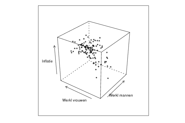
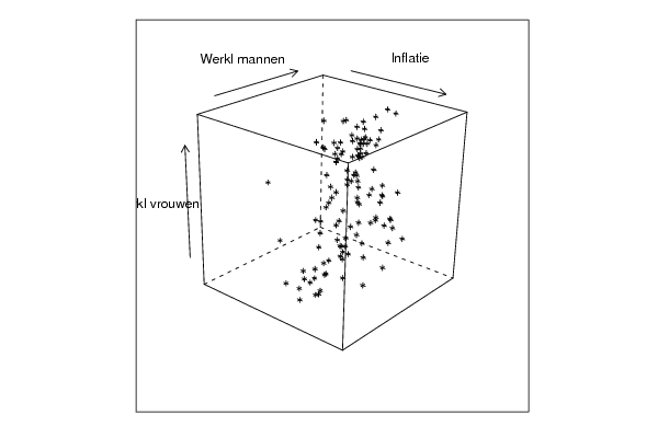
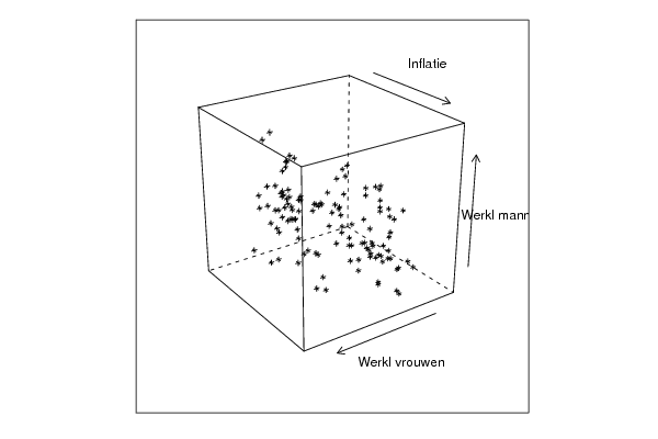
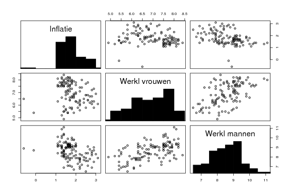
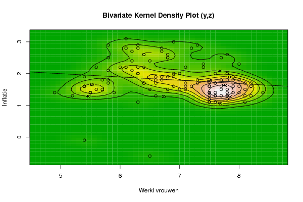
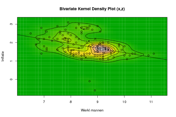
| Title produced by software | Trivariate Scatterplots | ||||||||||||||||||||
| Date of computation | Sat, 18 Dec 2010 16:57:07 +0000 | ||||||||||||||||||||
| Cite this page as follows | Statistical Computations at FreeStatistics.org, Office for Research Development and Education, URL https://freestatistics.org/blog/index.php?v=date/2010/Dec/18/t1292691477mcdxmkq4xvixihy.htm/, Retrieved Tue, 30 Apr 2024 02:13:14 +0000 | ||||||||||||||||||||
| Statistical Computations at FreeStatistics.org, Office for Research Development and Education, URL https://freestatistics.org/blog/index.php?pk=112109, Retrieved Tue, 30 Apr 2024 02:13:14 +0000 | |||||||||||||||||||||
| QR Codes: | |||||||||||||||||||||
|
| |||||||||||||||||||||
| Original text written by user: | |||||||||||||||||||||
| IsPrivate? | No (this computation is public) | ||||||||||||||||||||
| User-defined keywords | |||||||||||||||||||||
| Estimated Impact | 161 | ||||||||||||||||||||
Tree of Dependent Computations | |||||||||||||||||||||
| Family? (F = Feedback message, R = changed R code, M = changed R Module, P = changed Parameters, D = changed Data) | |||||||||||||||||||||
| F [Univariate Data Series] [HPC Retail Sales] [2008-03-02 15:42:48] [74be16979710d4c4e7c6647856088456] - MPD [Univariate Data Series] [WS8 1] [2010-11-30 15:47:30] [07a238a5afc23eb944f8545182f29d5a] - RMP [Classical Decomposition] [WS8 2] [2010-11-30 15:54:02] [07a238a5afc23eb944f8545182f29d5a] - RMPD [Univariate Data Series] [Statistiek: Werkl...] [2010-12-12 15:20:09] [07a238a5afc23eb944f8545182f29d5a] - D [Univariate Data Series] [Statistiek: Werkl...] [2010-12-14 09:08:05] [07a238a5afc23eb944f8545182f29d5a] - [Univariate Data Series] [Statistiek: Werkl...] [2010-12-14 09:12:36] [07a238a5afc23eb944f8545182f29d5a] - RMPD [Univariate Explorative Data Analysis] [Statistiek: U EDA...] [2010-12-17 19:07:44] [07a238a5afc23eb944f8545182f29d5a] - RMP [Central Tendency] [Statistiek: centr...] [2010-12-18 09:18:46] [07a238a5afc23eb944f8545182f29d5a] - RMP [Harrell-Davis Quantiles] [Statistiek: betro...] [2010-12-18 10:06:35] [07a238a5afc23eb944f8545182f29d5a] - RMPD [Bivariate Explorative Data Analysis] [statistiek: Bivar...] [2010-12-18 13:22:48] [07a238a5afc23eb944f8545182f29d5a] - RMPD [Pearson Correlation] [statistiek: pears...] [2010-12-18 14:12:28] [07a238a5afc23eb944f8545182f29d5a] - [Pearson Correlation] [statistiek: pears...] [2010-12-18 14:15:15] [07a238a5afc23eb944f8545182f29d5a] - RMPD [Trivariate Scatterplots] [Statistiek trivar...] [2010-12-18 16:57:07] [67e3c2d70de1dbb070b545ca6c893d5e] [Current] - PD [Trivariate Scatterplots] [Statistiek: triva...] [2010-12-18 17:03:13] [07a238a5afc23eb944f8545182f29d5a] - RMPD [Multiple Regression] [statistiek Multip...] [2010-12-18 19:03:25] [07a238a5afc23eb944f8545182f29d5a] - D [Multiple Regression] [statistiek Multip...] [2010-12-18 19:19:51] [07a238a5afc23eb944f8545182f29d5a] - D [Multiple Regression] [statistiek Multip...] [2010-12-18 19:32:07] [07a238a5afc23eb944f8545182f29d5a] | |||||||||||||||||||||
| Feedback Forum | |||||||||||||||||||||
Post a new message | |||||||||||||||||||||
Dataset | |||||||||||||||||||||
| Dataseries X: | |||||||||||||||||||||
8.9 8.4 8.1 8.3 8.1 8 8.7 9.2 9 8.9 8.5 8.1 7.5 7.1 6.9 7.1 7 6.7 7 7.3 7.7 8.4 8.4 8.8 9.1 9 8.6 7.9 7.7 7.8 9.2 9.4 9.2 8.7 8.4 8.6 9 9.1 8.7 8.2 7.9 7.9 9.1 9.4 9.4 9.1 9 9.3 9.9 9.8 9.3 8.3 8 8.5 10.4 11.1 10.9 10 9.2 9.2 9.5 9.6 9.5 9.1 8.9 9 10.1 10.3 10.2 9.6 9.2 9.3 9.4 9.4 9.2 9 9 9 9.8 10 9.8 9.3 9 9 9.1 9.1 9.1 9.2 8.8 8.3 8.4 8.1 7.7 7.9 7.9 8 7.9 7.6 7.1 6.8 6.5 6.9 8.2 8.7 8.3 7.9 7.5 7.8 8.3 8.4 8.2 7.6 7.2 7.5 8.7 9 8.6 7.9 7.8 8.2 | |||||||||||||||||||||
| Dataseries Y: | |||||||||||||||||||||
6.5 6.3 5.9 5.5 5.2 4.9 5.4 5.8 5.7 5.6 5.5 5.4 5.4 5.4 5.5 5.8 5.7 5.4 5.6 5.8 6.2 6.8 6.7 6.7 6.4 6.3 6.3 6.4 6.3 6 6.3 6.3 6.6 7.5 7.8 7.9 7.8 7.6 7.5 7.6 7.5 7.3 7.6 7.5 7.6 7.9 7.9 8.1 8.2 8 7.5 6.8 6.5 6.6 7.6 8 8.1 7.7 7.5 7.6 7.8 7.8 7.8 7.5 7.5 7.1 7.5 7.5 7.6 7.7 7.7 7.9 8.1 8.2 8.2 8.2 7.9 7.3 6.9 6.6 6.7 6.9 7 7.1 7.2 7.1 6.9 7 6.8 6.4 6.7 6.6 6.4 6.3 6.2 6.5 6.8 6.8 6.4 6.1 5.8 6.1 7.2 7.3 6.9 6.1 5.8 6.2 7.1 7.7 8 7.8 7.4 7.4 7.7 7.8 7.8 8 8.1 8.4 | |||||||||||||||||||||
| Dataseries Z: | |||||||||||||||||||||
-0.6 1.1 1.4 1.4 1.3 1.4 -0.1 1.8 1.5 1.5 1.4 1.6 1.6 1.6 1.4 1.7 1.8 1.9 2.2 2.1 2.4 2.6 2.8 2.7 2.6 2.9 2.8 2.2 2.2 2.2 2 2 1.7 1.4 1.3 1.4 1.3 1.3 1.4 2 1.7 1.8 1.7 1.6 1.7 1.9 1.8 1.7 1.6 1.8 1.6 1.5 1.5 1.3 1.4 1.4 1.3 1.3 1.2 1.1 1.4 1.2 1.5 1.1 1.3 1.5 1.1 1.4 1.3 1.5 1.6 1.7 1.1 1.6 1.3 1.7 1.6 1.7 1.9 1.8 1.9 1.6 1.5 1.6 1.6 1.7 2 2 1.9 1.7 1.8 1.9 1.7 2 2.1 2.4 2.5 2.5 2.6 2.2 2.5 2.8 2.8 2.9 3 3.1 2.9 2.7 2.2 2.5 2.3 2.6 2.3 2.2 1.8 1.8 2 1.6 1.5 1.4 | |||||||||||||||||||||
Tables (Output of Computation) | |||||||||||||||||||||
| |||||||||||||||||||||
Figures (Output of Computation) | |||||||||||||||||||||
Input Parameters & R Code | |||||||||||||||||||||
| Parameters (Session): | |||||||||||||||||||||
| par1 = 50 ; par2 = 50 ; par3 = Y ; par4 = Y ; par5 = Werkl mannen ; par6 = Werkl vrouwen ; par7 = Inflatie ; | |||||||||||||||||||||
| Parameters (R input): | |||||||||||||||||||||
| par1 = 50 ; par2 = 50 ; par3 = Y ; par4 = Y ; par5 = Werkl mannen ; par6 = Werkl vrouwen ; par7 = Inflatie ; | |||||||||||||||||||||
| R code (references can be found in the software module): | |||||||||||||||||||||
x <- array(x,dim=c(length(x),1)) | |||||||||||||||||||||