Free Statistics
of Irreproducible Research!
Description of Statistical Computation | |||||||||||||||||||||||||||||||||||||||||||||||||||||||||||||
|---|---|---|---|---|---|---|---|---|---|---|---|---|---|---|---|---|---|---|---|---|---|---|---|---|---|---|---|---|---|---|---|---|---|---|---|---|---|---|---|---|---|---|---|---|---|---|---|---|---|---|---|---|---|---|---|---|---|---|---|---|---|
| Author's title | |||||||||||||||||||||||||||||||||||||||||||||||||||||||||||||
| Author | *The author of this computation has been verified* | ||||||||||||||||||||||||||||||||||||||||||||||||||||||||||||
| R Software Module | rwasp_linear_regression.wasp | ||||||||||||||||||||||||||||||||||||||||||||||||||||||||||||
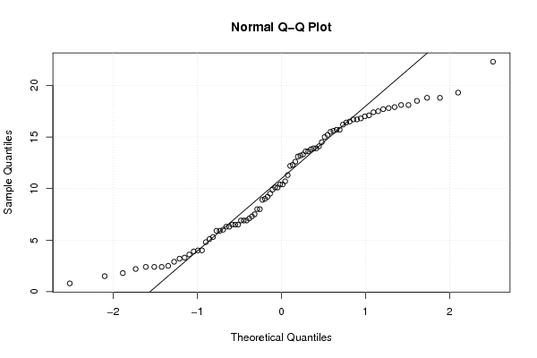
| Title produced by software | Linear Regression Graphical Model Validation | ||||||||||||||||||||||||||||||||||||||||||||||||||||||||||||
| Date of computation | Sat, 18 Dec 2010 15:56:52 +0000 | ||||||||||||||||||||||||||||||||||||||||||||||||||||||||||||
| Cite this page as follows | Statistical Computations at FreeStatistics.org, Office for Research Development and Education, URL https://freestatistics.org/blog/index.php?v=date/2010/Dec/18/t12926877458pdf6ggr5qzqmrk.htm/, Retrieved Tue, 30 Apr 2024 04:22:44 +0000 | ||||||||||||||||||||||||||||||||||||||||||||||||||||||||||||
| Statistical Computations at FreeStatistics.org, Office for Research Development and Education, URL https://freestatistics.org/blog/index.php?pk=112069, Retrieved Tue, 30 Apr 2024 04:22:44 +0000 | |||||||||||||||||||||||||||||||||||||||||||||||||||||||||||||
| QR Codes: | |||||||||||||||||||||||||||||||||||||||||||||||||||||||||||||
|
| |||||||||||||||||||||||||||||||||||||||||||||||||||||||||||||
| Original text written by user: | |||||||||||||||||||||||||||||||||||||||||||||||||||||||||||||
| IsPrivate? | No (this computation is public) | ||||||||||||||||||||||||||||||||||||||||||||||||||||||||||||
| User-defined keywords | |||||||||||||||||||||||||||||||||||||||||||||||||||||||||||||
| Estimated Impact | 144 | ||||||||||||||||||||||||||||||||||||||||||||||||||||||||||||
Tree of Dependent Computations | |||||||||||||||||||||||||||||||||||||||||||||||||||||||||||||
| Family? (F = Feedback message, R = changed R code, M = changed R Module, P = changed Parameters, D = changed Data) | |||||||||||||||||||||||||||||||||||||||||||||||||||||||||||||
| - [Linear Regression Graphical Model Validation] [Colombia Coffee -...] [2008-02-26 10:22:06] [74be16979710d4c4e7c6647856088456] - M D [Linear Regression Graphical Model Validation] [ass 3 ws6] [2010-11-14 10:45:24] [0e7b3997dca5cf9d94982fb4db7bd3d5] - D [Linear Regression Graphical Model Validation] [mini tutorial] [2010-11-16 09:49:54] [0e7b3997dca5cf9d94982fb4db7bd3d5] - D [Linear Regression Graphical Model Validation] [Huwelijken vs Tem...] [2010-12-18 15:56:52] [3f56c8f677e988de577e4e00a8180a48] [Current] | |||||||||||||||||||||||||||||||||||||||||||||||||||||||||||||
| Feedback Forum | |||||||||||||||||||||||||||||||||||||||||||||||||||||||||||||
Post a new message | |||||||||||||||||||||||||||||||||||||||||||||||||||||||||||||
Dataset | |||||||||||||||||||||||||||||||||||||||||||||||||||||||||||||
| Dataseries X: | |||||||||||||||||||||||||||||||||||||||||||||||||||||||||||||
2,5 1,8 7,3 9,9 13,2 17,8 18,8 19,3 13,9 7,5 8 4 3,6 4,8 5,9 10,4 12,3 15,5 16,7 18,8 15,2 11,3 6,3 3,2 5,3 2,4 6,5 10,4 12,6 16,8 17,7 16,2 15,7 13,3 6,9 4 1,5 2,9 3,9 9 14,5 16,7 22,3 16,4 17,9 13,6 9,2 6,5 7,1 6 8 13,1 14,1 17,5 17 17,1 13,8 10,1 6,9 2,4 6,5 5,1 5,9 8,9 15,7 16,5 18,1 17,4 13,6 10,1 6,9 2,4 0,8 3,3 6,3 12,2 13,9 15,6 18,1 18,5 15 10,7 9,5 2,2 | |||||||||||||||||||||||||||||||||||||||||||||||||||||||||||||
| Dataseries Y: | |||||||||||||||||||||||||||||||||||||||||||||||||||||||||||||
3111 3995 5245 5588 10681 10516 7496 9935 10249 6271 3616 3724 2886 3318 4166 6401 9209 9820 7470 8207 9564 5309 3385 3706 2733 3045 3449 5542 10072 9418 7516 7840 10081 4956 3641 3970 2931 3170 3889 4850 8037 12370 6712 7297 10613 5184 3506 3810 2692 3073 3713 4555 7807 10869 9682 7704 9826 5456 3677 3431 2765 3483 3445 6081 8767 9407 6551 12480 9530 5960 3252 3717 2642 2989 3607 5366 8898 9435 7328 8594 11349 5797 3621 3851 | |||||||||||||||||||||||||||||||||||||||||||||||||||||||||||||
Tables (Output of Computation) | |||||||||||||||||||||||||||||||||||||||||||||||||||||||||||||
| |||||||||||||||||||||||||||||||||||||||||||||||||||||||||||||
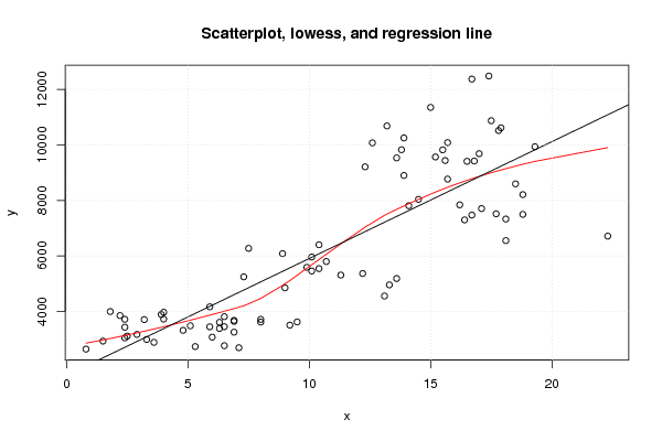
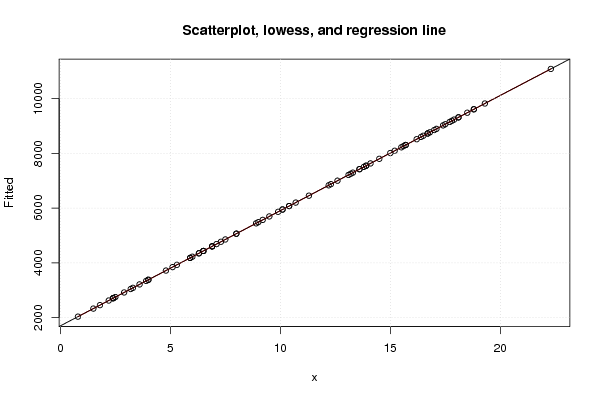
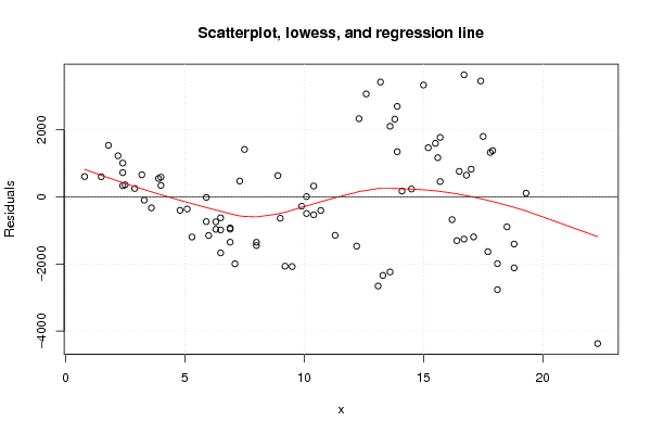
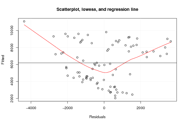
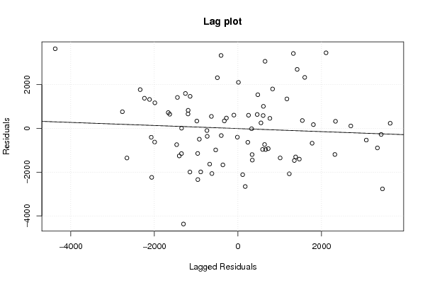
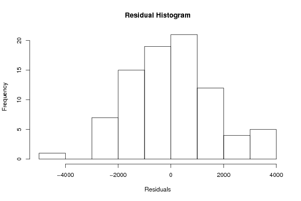
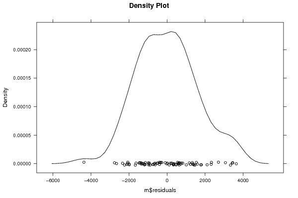
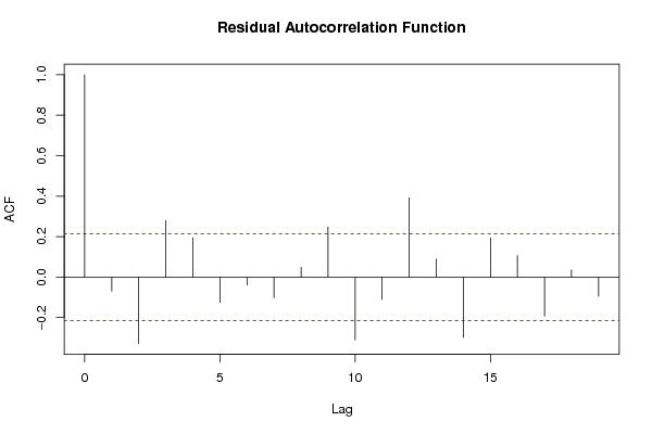
Figures (Output of Computation) | |||||||||||||||||||||||||||||||||||||||||||||||||||||||||||||
Input Parameters & R Code | |||||||||||||||||||||||||||||||||||||||||||||||||||||||||||||
| Parameters (Session): | |||||||||||||||||||||||||||||||||||||||||||||||||||||||||||||
| par1 = 0 ; | |||||||||||||||||||||||||||||||||||||||||||||||||||||||||||||
| Parameters (R input): | |||||||||||||||||||||||||||||||||||||||||||||||||||||||||||||
| par1 = 0 ; | |||||||||||||||||||||||||||||||||||||||||||||||||||||||||||||
| R code (references can be found in the software module): | |||||||||||||||||||||||||||||||||||||||||||||||||||||||||||||
par1 <- as.numeric(par1) | |||||||||||||||||||||||||||||||||||||||||||||||||||||||||||||