Free Statistics
of Irreproducible Research!
Description of Statistical Computation | |||||||||||||||||||||||||||||||||||||||||||||||||||||
|---|---|---|---|---|---|---|---|---|---|---|---|---|---|---|---|---|---|---|---|---|---|---|---|---|---|---|---|---|---|---|---|---|---|---|---|---|---|---|---|---|---|---|---|---|---|---|---|---|---|---|---|---|---|
| Author's title | |||||||||||||||||||||||||||||||||||||||||||||||||||||
| Author | *The author of this computation has been verified* | ||||||||||||||||||||||||||||||||||||||||||||||||||||
| R Software Module | rwasp_edauni.wasp | ||||||||||||||||||||||||||||||||||||||||||||||||||||
| Title produced by software | Univariate Explorative Data Analysis | ||||||||||||||||||||||||||||||||||||||||||||||||||||
| Date of computation | Sat, 18 Dec 2010 15:10:03 +0000 | ||||||||||||||||||||||||||||||||||||||||||||||||||||
| Cite this page as follows | Statistical Computations at FreeStatistics.org, Office for Research Development and Education, URL https://freestatistics.org/blog/index.php?v=date/2010/Dec/18/t12926850619k2z74rdqpxcpoe.htm/, Retrieved Tue, 30 Apr 2024 06:18:38 +0000 | ||||||||||||||||||||||||||||||||||||||||||||||||||||
| Statistical Computations at FreeStatistics.org, Office for Research Development and Education, URL https://freestatistics.org/blog/index.php?pk=112026, Retrieved Tue, 30 Apr 2024 06:18:38 +0000 | |||||||||||||||||||||||||||||||||||||||||||||||||||||
| QR Codes: | |||||||||||||||||||||||||||||||||||||||||||||||||||||
|
| |||||||||||||||||||||||||||||||||||||||||||||||||||||
| Original text written by user: | |||||||||||||||||||||||||||||||||||||||||||||||||||||
| IsPrivate? | No (this computation is public) | ||||||||||||||||||||||||||||||||||||||||||||||||||||
| User-defined keywords | |||||||||||||||||||||||||||||||||||||||||||||||||||||
| Estimated Impact | 164 | ||||||||||||||||||||||||||||||||||||||||||||||||||||
Tree of Dependent Computations | |||||||||||||||||||||||||||||||||||||||||||||||||||||
| Family? (F = Feedback message, R = changed R code, M = changed R Module, P = changed Parameters, D = changed Data) | |||||||||||||||||||||||||||||||||||||||||||||||||||||
| - [Univariate Data Series] [WS2] [2009-10-12 16:56:43] [4f76e114ed5e444b1133aad392380aad] - RMPD [Univariate Explorative Data Analysis] [Paper EDA Calculator] [2010-12-18 15:10:03] [33ba4313a043c7c916d0d88da7cd101b] [Current] - RMP [Central Tendency] [Paper CT Verkeers...] [2010-12-19 15:11:24] [abf4ff90b26c6b37be4a30063b404639] - RMPD [Central Tendency] [Paper CT Auto Ins...] [2010-12-19 15:15:16] [abf4ff90b26c6b37be4a30063b404639] - D [Univariate Explorative Data Analysis] [] [2010-12-24 15:18:46] [dd4fe494cff2ee46c12b15bdc7b848ca] - RMPD [Histogram and QQPlot (Reddy-Moores Data)] [] [2010-12-24 15:38:57] [dd4fe494cff2ee46c12b15bdc7b848ca] - RMPD [Histogram and QQPlot (Reddy-Moores Data)] [] [2010-12-24 15:42:08] [dd4fe494cff2ee46c12b15bdc7b848ca] - RMPD [Histogram and QQPlot (Reddy-Moores Data)] [] [2010-12-24 15:43:22] [dd4fe494cff2ee46c12b15bdc7b848ca] | |||||||||||||||||||||||||||||||||||||||||||||||||||||
| Feedback Forum | |||||||||||||||||||||||||||||||||||||||||||||||||||||
Post a new message | |||||||||||||||||||||||||||||||||||||||||||||||||||||
Dataset | |||||||||||||||||||||||||||||||||||||||||||||||||||||
| Dataseries X: | |||||||||||||||||||||||||||||||||||||||||||||||||||||
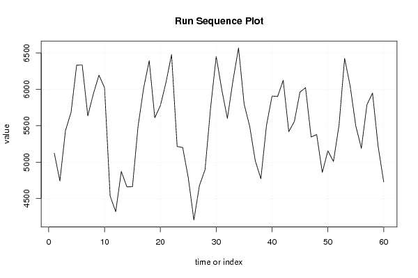
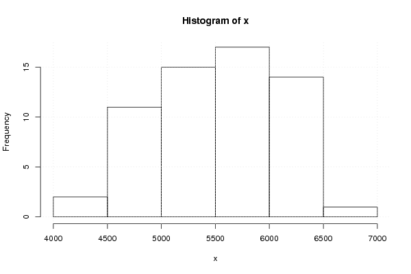
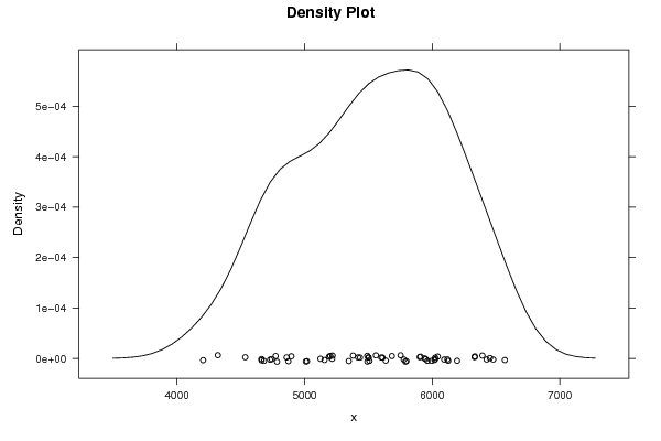
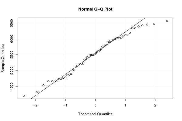
5124 4742 5434 5684 6332 6334 5636 5940 6195 6022 4535 4320 4872 4662 4663 5491 6018 6393 5610 5777 6094 6478 5216 5201 4784 4205 4681 4896 5752 6452 5995 5601 6119 6569 5798 5492 5018 4773 5502 5908 5902 6125 5419 5559 5962 6023 5346 5379 4859 5156 5010 5508 6426 6043 5499 5191 5790 5949 5219 4729 | |||||||||||||||||||||||||||||||||||||||||||||||||||||
Tables (Output of Computation) | |||||||||||||||||||||||||||||||||||||||||||||||||||||
| |||||||||||||||||||||||||||||||||||||||||||||||||||||
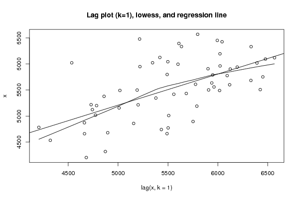
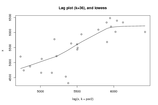
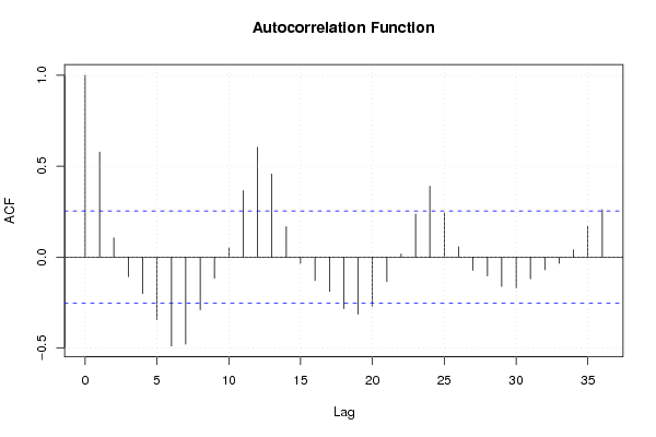
Figures (Output of Computation) | |||||||||||||||||||||||||||||||||||||||||||||||||||||
Input Parameters & R Code | |||||||||||||||||||||||||||||||||||||||||||||||||||||
| Parameters (Session): | |||||||||||||||||||||||||||||||||||||||||||||||||||||
| par1 = 0 ; par2 = 36 ; | |||||||||||||||||||||||||||||||||||||||||||||||||||||
| Parameters (R input): | |||||||||||||||||||||||||||||||||||||||||||||||||||||
| par1 = 0 ; par2 = 36 ; | |||||||||||||||||||||||||||||||||||||||||||||||||||||
| R code (references can be found in the software module): | |||||||||||||||||||||||||||||||||||||||||||||||||||||
par1 <- as.numeric(par1) | |||||||||||||||||||||||||||||||||||||||||||||||||||||