Free Statistics
of Irreproducible Research!
Description of Statistical Computation | |||||||||||||||||||||||||||||||||||||||||||||||||||||
|---|---|---|---|---|---|---|---|---|---|---|---|---|---|---|---|---|---|---|---|---|---|---|---|---|---|---|---|---|---|---|---|---|---|---|---|---|---|---|---|---|---|---|---|---|---|---|---|---|---|---|---|---|---|
| Author's title | |||||||||||||||||||||||||||||||||||||||||||||||||||||
| Author | *The author of this computation has been verified* | ||||||||||||||||||||||||||||||||||||||||||||||||||||
| R Software Module | rwasp_edauni.wasp | ||||||||||||||||||||||||||||||||||||||||||||||||||||
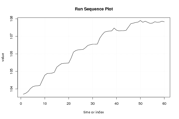
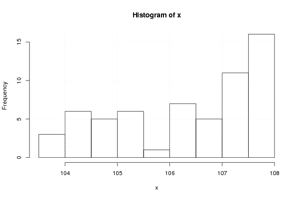
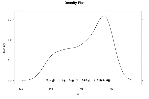
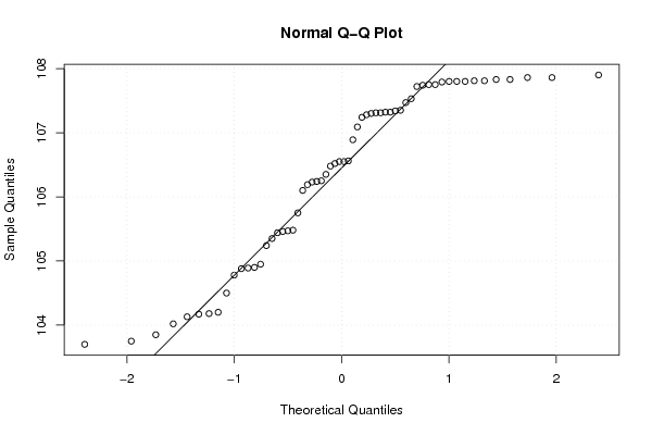
| Title produced by software | Univariate Explorative Data Analysis | ||||||||||||||||||||||||||||||||||||||||||||||||||||
| Date of computation | Sat, 18 Dec 2010 13:35:49 +0000 | ||||||||||||||||||||||||||||||||||||||||||||||||||||
| Cite this page as follows | Statistical Computations at FreeStatistics.org, Office for Research Development and Education, URL https://freestatistics.org/blog/index.php?v=date/2010/Dec/18/t129268082306l7yv1ks19awkh.htm/, Retrieved Thu, 03 Jul 2025 06:28:20 +0000 | ||||||||||||||||||||||||||||||||||||||||||||||||||||
| Statistical Computations at FreeStatistics.org, Office for Research Development and Education, URL https://freestatistics.org/blog/index.php?pk=111973, Retrieved Thu, 03 Jul 2025 06:28:20 +0000 | |||||||||||||||||||||||||||||||||||||||||||||||||||||
| QR Codes: | |||||||||||||||||||||||||||||||||||||||||||||||||||||
|
| |||||||||||||||||||||||||||||||||||||||||||||||||||||
| Original text written by user: | |||||||||||||||||||||||||||||||||||||||||||||||||||||
| IsPrivate? | No (this computation is public) | ||||||||||||||||||||||||||||||||||||||||||||||||||||
| User-defined keywords | |||||||||||||||||||||||||||||||||||||||||||||||||||||
| Estimated Impact | 248 | ||||||||||||||||||||||||||||||||||||||||||||||||||||
Tree of Dependent Computations | |||||||||||||||||||||||||||||||||||||||||||||||||||||
| Family? (F = Feedback message, R = changed R code, M = changed R Module, P = changed Parameters, D = changed Data) | |||||||||||||||||||||||||||||||||||||||||||||||||||||
| - [Univariate Data Series] [Univariate Time S...] [2009-10-12 09:36:05] [6e4e01d7eb22a9f33d58ebb35753a195] - RMPD [Univariate Explorative Data Analysis] [Paper Yt] [2010-12-18 13:35:49] [9ac5e967b06232cfb69e0c18e3cc2b37] [Current] - D [Univariate Explorative Data Analysis] [Horeca run sequen...] [2010-12-22 14:30:44] [a9e130f95bad0a0597234e75c6380c5a] - D [Univariate Explorative Data Analysis] [] [2011-12-20 17:02:38] [06f5daa9a1979410bf169cb7a41fb3eb] | |||||||||||||||||||||||||||||||||||||||||||||||||||||
| Feedback Forum | |||||||||||||||||||||||||||||||||||||||||||||||||||||
Post a new message | |||||||||||||||||||||||||||||||||||||||||||||||||||||
Dataset | |||||||||||||||||||||||||||||||||||||||||||||||||||||
| Dataseries X: | |||||||||||||||||||||||||||||||||||||||||||||||||||||
103.7 103.75 103.85 104.02 104.13 104.17 104.18 104.2 104.5 104.78 104.88 104.89 104.9 104.95 105.24 105.35 105.44 105.46 105.47 105.48 105.75 106.1 106.19 106.23 106.24 106.25 106.35 106.48 106.52 106.55 106.55 106.56 106.89 107.09 107.24 107.28 107.3 107.31 107.47 107.35 107.31 107.32 107.32 107.34 107.53 107.72 107.75 107.79 107.81 107.9 107.8 107.86 107.8 107.74 107.75 107.83 107.8 107.81 107.86 107.83 | |||||||||||||||||||||||||||||||||||||||||||||||||||||
Tables (Output of Computation) | |||||||||||||||||||||||||||||||||||||||||||||||||||||
| |||||||||||||||||||||||||||||||||||||||||||||||||||||
Figures (Output of Computation) | |||||||||||||||||||||||||||||||||||||||||||||||||||||
Input Parameters & R Code | |||||||||||||||||||||||||||||||||||||||||||||||||||||
| Parameters (Session): | |||||||||||||||||||||||||||||||||||||||||||||||||||||
| par1 = 0 ; par2 = 0 ; | |||||||||||||||||||||||||||||||||||||||||||||||||||||
| Parameters (R input): | |||||||||||||||||||||||||||||||||||||||||||||||||||||
| par1 = 0 ; par2 = 0 ; | |||||||||||||||||||||||||||||||||||||||||||||||||||||
| R code (references can be found in the software module): | |||||||||||||||||||||||||||||||||||||||||||||||||||||
par1 <- as.numeric(par1) | |||||||||||||||||||||||||||||||||||||||||||||||||||||