library(lattice)
library(lmtest)
n25 <- 25 #minimum number of obs. for Goldfeld-Quandt test
par1 <- as.numeric(par1)
x <- t(y)
k <- length(x[1,])
n <- length(x[,1])
x1 <- cbind(x[,par1], x[,1:k!=par1])
mycolnames <- c(colnames(x)[par1], colnames(x)[1:k!=par1])
colnames(x1) <- mycolnames #colnames(x)[par1]
x <- x1
if (par3 == 'First Differences'){
x2 <- array(0, dim=c(n-1,k), dimnames=list(1:(n-1), paste('(1-B)',colnames(x),sep='')))
for (i in 1:n-1) {
for (j in 1:k) {
x2[i,j] <- x[i+1,j] - x[i,j]
}
}
x <- x2
}
if (par2 == 'Include Monthly Dummies'){
x2 <- array(0, dim=c(n,11), dimnames=list(1:n, paste('M', seq(1:11), sep ='')))
for (i in 1:11){
x2[seq(i,n,12),i] <- 1
}
x <- cbind(x, x2)
}
if (par2 == 'Include Quarterly Dummies'){
x2 <- array(0, dim=c(n,3), dimnames=list(1:n, paste('Q', seq(1:3), sep ='')))
for (i in 1:3){
x2[seq(i,n,4),i] <- 1
}
x <- cbind(x, x2)
}
k <- length(x[1,])
if (par3 == 'Linear Trend'){
x <- cbind(x, c(1:n))
colnames(x)[k+1] <- 't'
}
x
k <- length(x[1,])
df <- as.data.frame(x)
(mylm <- lm(df))
(mysum <- summary(mylm))
if (n > n25) {
kp3 <- k + 3
nmkm3 <- n - k - 3
gqarr <- array(NA, dim=c(nmkm3-kp3+1,3))
numgqtests <- 0
numsignificant1 <- 0
numsignificant5 <- 0
numsignificant10 <- 0
for (mypoint in kp3:nmkm3) {
j <- 0
numgqtests <- numgqtests + 1
for (myalt in c('greater', 'two.sided', 'less')) {
j <- j + 1
gqarr[mypoint-kp3+1,j] <- gqtest(mylm, point=mypoint, alternative=myalt)$p.value
}
if (gqarr[mypoint-kp3+1,2] < 0.01) numsignificant1 <- numsignificant1 + 1
if (gqarr[mypoint-kp3+1,2] < 0.05) numsignificant5 <- numsignificant5 + 1
if (gqarr[mypoint-kp3+1,2] < 0.10) numsignificant10 <- numsignificant10 + 1
}
gqarr
}
bitmap(file='test0.png')
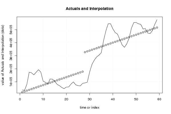
plot(x[,1], type='l', main='Actuals and Interpolation', ylab='value of Actuals and Interpolation (dots)', xlab='time or index')
points(x[,1]-mysum$resid)
grid()
dev.off()
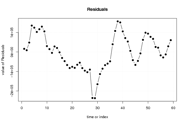
bitmap(file='test1.png')
plot(mysum$resid, type='b', pch=19, main='Residuals', ylab='value of Residuals', xlab='time or index')
grid()
dev.off()
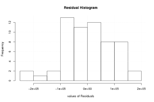
bitmap(file='test2.png')
hist(mysum$resid, main='Residual Histogram', xlab='values of Residuals')
grid()
dev.off()
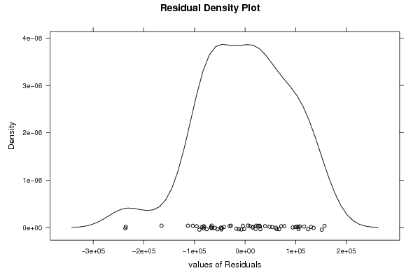
bitmap(file='test3.png')
densityplot(~mysum$resid,col='black',main='Residual Density Plot', xlab='values of Residuals')
dev.off()
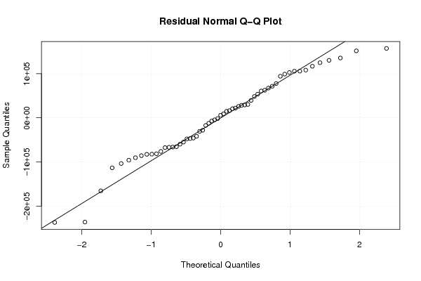
bitmap(file='test4.png')
qqnorm(mysum$resid, main='Residual Normal Q-Q Plot')
qqline(mysum$resid)
grid()
dev.off()
(myerror <- as.ts(mysum$resid))
bitmap(file='test5.png')
dum <- cbind(lag(myerror,k=1),myerror)
dum
dum1 <- dum[2:length(myerror),]
dum1
z <- as.data.frame(dum1)
z
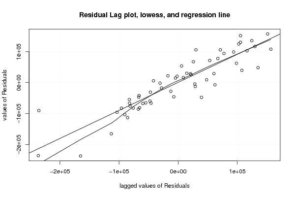
plot(z,main=paste('Residual Lag plot, lowess, and regression line'), ylab='values of Residuals', xlab='lagged values of Residuals')
lines(lowess(z))
abline(lm(z))
grid()
dev.off()
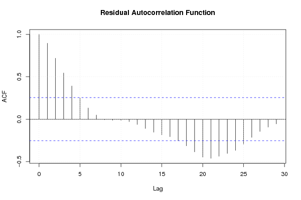
bitmap(file='test6.png')
acf(mysum$resid, lag.max=length(mysum$resid)/2, main='Residual Autocorrelation Function')
grid()
dev.off()
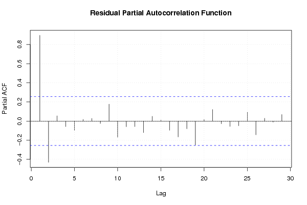
bitmap(file='test7.png')
pacf(mysum$resid, lag.max=length(mysum$resid)/2, main='Residual Partial Autocorrelation Function')
grid()
dev.off()
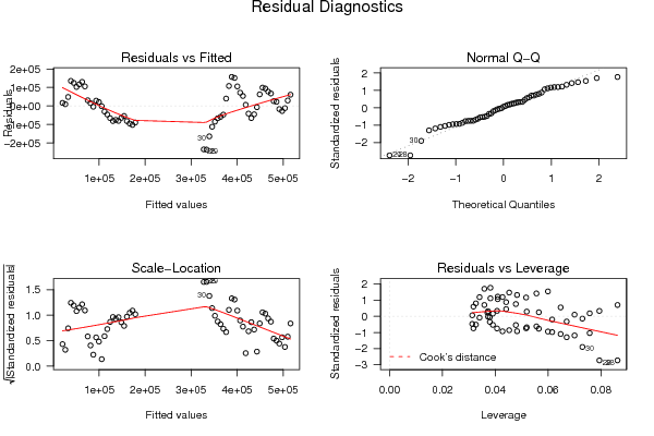
bitmap(file='test8.png')
opar <- par(mfrow = c(2,2), oma = c(0, 0, 1.1, 0))
plot(mylm, las = 1, sub='Residual Diagnostics')
par(opar)
dev.off()
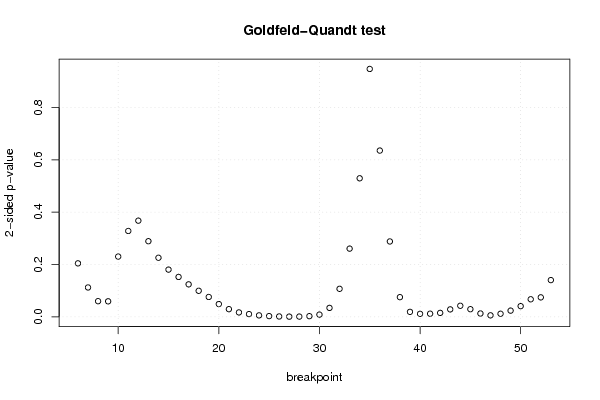
if (n > n25) {
bitmap(file='test9.png')
plot(kp3:nmkm3,gqarr[,2], main='Goldfeld-Quandt test',ylab='2-sided p-value',xlab='breakpoint')
grid()
dev.off()
}
load(file='createtable')
a<-table.start()
a<-table.row.start(a)
a<-table.element(a, 'Multiple Linear Regression - Estimated Regression Equation', 1, TRUE)
a<-table.row.end(a)
myeq <- colnames(x)[1]
myeq <- paste(myeq, '[t] = ', sep='')
for (i in 1:k){
if (mysum$coefficients[i,1] > 0) myeq <- paste(myeq, '+', '')
myeq <- paste(myeq, mysum$coefficients[i,1], sep=' ')
if (rownames(mysum$coefficients)[i] != '(Intercept)') {
myeq <- paste(myeq, rownames(mysum$coefficients)[i], sep='')
if (rownames(mysum$coefficients)[i] != 't') myeq <- paste(myeq, '[t]', sep='')
}
}
myeq <- paste(myeq, ' + e[t]')
a<-table.row.start(a)
a<-table.element(a, myeq)
a<-table.row.end(a)
a<-table.end(a)
table.save(a,file='mytable1.tab')
a<-table.start()
a<-table.row.start(a)
a<-table.element(a,hyperlink('ols1.htm','Multiple Linear Regression - Ordinary Least Squares',''), 6, TRUE)
a<-table.row.end(a)
a<-table.row.start(a)
a<-table.element(a,'Variable',header=TRUE)
a<-table.element(a,'Parameter',header=TRUE)
a<-table.element(a,'S.D.',header=TRUE)
a<-table.element(a,'T-STAT
H0: parameter = 0',header=TRUE)
a<-table.element(a,'2-tail p-value',header=TRUE)
a<-table.element(a,'1-tail p-value',header=TRUE)
a<-table.row.end(a)
for (i in 1:k){
a<-table.row.start(a)
a<-table.element(a,rownames(mysum$coefficients)[i],header=TRUE)
a<-table.element(a,mysum$coefficients[i,1])
a<-table.element(a, round(mysum$coefficients[i,2],6))
a<-table.element(a, round(mysum$coefficients[i,3],4))
a<-table.element(a, round(mysum$coefficients[i,4],6))
a<-table.element(a, round(mysum$coefficients[i,4]/2,6))
a<-table.row.end(a)
}
a<-table.end(a)
table.save(a,file='mytable2.tab')
a<-table.start()
a<-table.row.start(a)
a<-table.element(a, 'Multiple Linear Regression - Regression Statistics', 2, TRUE)
a<-table.row.end(a)
a<-table.row.start(a)
a<-table.element(a, 'Multiple R',1,TRUE)
a<-table.element(a, sqrt(mysum$r.squared))
a<-table.row.end(a)
a<-table.row.start(a)
a<-table.element(a, 'R-squared',1,TRUE)
a<-table.element(a, mysum$r.squared)
a<-table.row.end(a)
a<-table.row.start(a)
a<-table.element(a, 'Adjusted R-squared',1,TRUE)
a<-table.element(a, mysum$adj.r.squared)
a<-table.row.end(a)
a<-table.row.start(a)
a<-table.element(a, 'F-TEST (value)',1,TRUE)
a<-table.element(a, mysum$fstatistic[1])
a<-table.row.end(a)
a<-table.row.start(a)
a<-table.element(a, 'F-TEST (DF numerator)',1,TRUE)
a<-table.element(a, mysum$fstatistic[2])
a<-table.row.end(a)
a<-table.row.start(a)
a<-table.element(a, 'F-TEST (DF denominator)',1,TRUE)
a<-table.element(a, mysum$fstatistic[3])
a<-table.row.end(a)
a<-table.row.start(a)
a<-table.element(a, 'p-value',1,TRUE)
a<-table.element(a, 1-pf(mysum$fstatistic[1],mysum$fstatistic[2],mysum$fstatistic[3]))
a<-table.row.end(a)
a<-table.row.start(a)
a<-table.element(a, 'Multiple Linear Regression - Residual Statistics', 2, TRUE)
a<-table.row.end(a)
a<-table.row.start(a)
a<-table.element(a, 'Residual Standard Deviation',1,TRUE)
a<-table.element(a, mysum$sigma)
a<-table.row.end(a)
a<-table.row.start(a)
a<-table.element(a, 'Sum Squared Residuals',1,TRUE)
a<-table.element(a, sum(myerror*myerror))
a<-table.row.end(a)
a<-table.end(a)
table.save(a,file='mytable3.tab')
a<-table.start()
a<-table.row.start(a)
a<-table.element(a, 'Multiple Linear Regression - Actuals, Interpolation, and Residuals', 4, TRUE)
a<-table.row.end(a)
a<-table.row.start(a)
a<-table.element(a, 'Time or Index', 1, TRUE)
a<-table.element(a, 'Actuals', 1, TRUE)
a<-table.element(a, 'Interpolation
Forecast', 1, TRUE)
a<-table.element(a, 'Residuals
Prediction Error', 1, TRUE)
a<-table.row.end(a)
for (i in 1:n) {
a<-table.row.start(a)
a<-table.element(a,i, 1, TRUE)
a<-table.element(a,x[i])
a<-table.element(a,x[i]-mysum$resid[i])
a<-table.element(a,mysum$resid[i])
a<-table.row.end(a)
}
a<-table.end(a)
table.save(a,file='mytable4.tab')
if (n > n25) {
a<-table.start()
a<-table.row.start(a)
a<-table.element(a,'Goldfeld-Quandt test for Heteroskedasticity',4,TRUE)
a<-table.row.end(a)
a<-table.row.start(a)
a<-table.element(a,'p-values',header=TRUE)
a<-table.element(a,'Alternative Hypothesis',3,header=TRUE)
a<-table.row.end(a)
a<-table.row.start(a)
a<-table.element(a,'breakpoint index',header=TRUE)
a<-table.element(a,'greater',header=TRUE)
a<-table.element(a,'2-sided',header=TRUE)
a<-table.element(a,'less',header=TRUE)
a<-table.row.end(a)
for (mypoint in kp3:nmkm3) {
a<-table.row.start(a)
a<-table.element(a,mypoint,header=TRUE)
a<-table.element(a,gqarr[mypoint-kp3+1,1])
a<-table.element(a,gqarr[mypoint-kp3+1,2])
a<-table.element(a,gqarr[mypoint-kp3+1,3])
a<-table.row.end(a)
}
a<-table.end(a)
table.save(a,file='mytable5.tab')
a<-table.start()
a<-table.row.start(a)
a<-table.element(a,'Meta Analysis of Goldfeld-Quandt test for Heteroskedasticity',4,TRUE)
a<-table.row.end(a)
a<-table.row.start(a)
a<-table.element(a,'Description',header=TRUE)
a<-table.element(a,'# significant tests',header=TRUE)
a<-table.element(a,'% significant tests',header=TRUE)
a<-table.element(a,'OK/NOK',header=TRUE)
a<-table.row.end(a)
a<-table.row.start(a)
a<-table.element(a,'1% type I error level',header=TRUE)
a<-table.element(a,numsignificant1)
a<-table.element(a,numsignificant1/numgqtests)
if (numsignificant1/numgqtests < 0.01) dum <- 'OK' else dum <- 'NOK'
a<-table.element(a,dum)
a<-table.row.end(a)
a<-table.row.start(a)
a<-table.element(a,'5% type I error level',header=TRUE)
a<-table.element(a,numsignificant5)
a<-table.element(a,numsignificant5/numgqtests)
if (numsignificant5/numgqtests < 0.05) dum <- 'OK' else dum <- 'NOK'
a<-table.element(a,dum)
a<-table.row.end(a)
a<-table.row.start(a)
a<-table.element(a,'10% type I error level',header=TRUE)
a<-table.element(a,numsignificant10)
a<-table.element(a,numsignificant10/numgqtests)
if (numsignificant10/numgqtests < 0.1) dum <- 'OK' else dum <- 'NOK'
a<-table.element(a,dum)
a<-table.row.end(a)
a<-table.end(a)
table.save(a,file='mytable6.tab')
}
|