Free Statistics
of Irreproducible Research!
Description of Statistical Computation | |||||||||||||||||||||||||||||||||||||||||||||||||||||
|---|---|---|---|---|---|---|---|---|---|---|---|---|---|---|---|---|---|---|---|---|---|---|---|---|---|---|---|---|---|---|---|---|---|---|---|---|---|---|---|---|---|---|---|---|---|---|---|---|---|---|---|---|---|
| Author's title | |||||||||||||||||||||||||||||||||||||||||||||||||||||
| Author | *The author of this computation has been verified* | ||||||||||||||||||||||||||||||||||||||||||||||||||||
| R Software Module | rwasp_edauni.wasp | ||||||||||||||||||||||||||||||||||||||||||||||||||||
| Title produced by software | Univariate Explorative Data Analysis | ||||||||||||||||||||||||||||||||||||||||||||||||||||
| Date of computation | Thu, 16 Dec 2010 14:27:05 +0000 | ||||||||||||||||||||||||||||||||||||||||||||||||||||
| Cite this page as follows | Statistical Computations at FreeStatistics.org, Office for Research Development and Education, URL https://freestatistics.org/blog/index.php?v=date/2010/Dec/16/t12925095456kio057yql9zc2o.htm/, Retrieved Fri, 03 May 2024 14:44:29 +0000 | ||||||||||||||||||||||||||||||||||||||||||||||||||||
| Statistical Computations at FreeStatistics.org, Office for Research Development and Education, URL https://freestatistics.org/blog/index.php?pk=110961, Retrieved Fri, 03 May 2024 14:44:29 +0000 | |||||||||||||||||||||||||||||||||||||||||||||||||||||
| QR Codes: | |||||||||||||||||||||||||||||||||||||||||||||||||||||
|
| |||||||||||||||||||||||||||||||||||||||||||||||||||||
| Original text written by user: | |||||||||||||||||||||||||||||||||||||||||||||||||||||
| IsPrivate? | No (this computation is public) | ||||||||||||||||||||||||||||||||||||||||||||||||||||
| User-defined keywords | |||||||||||||||||||||||||||||||||||||||||||||||||||||
| Estimated Impact | 167 | ||||||||||||||||||||||||||||||||||||||||||||||||||||
Tree of Dependent Computations | |||||||||||||||||||||||||||||||||||||||||||||||||||||
| Family? (F = Feedback message, R = changed R code, M = changed R Module, P = changed Parameters, D = changed Data) | |||||||||||||||||||||||||||||||||||||||||||||||||||||
| - [(Partial) Autocorrelation Function] [] [2010-12-13 08:35:23] [21eff0c210342db4afbdafe426a7c254] - PD [(Partial) Autocorrelation Function] [] [2010-12-13 09:29:04] [21eff0c210342db4afbdafe426a7c254] - D [(Partial) Autocorrelation Function] [] [2010-12-13 10:05:17] [21eff0c210342db4afbdafe426a7c254] - RM D [ARIMA Forecasting] [] [2010-12-13 10:48:48] [21eff0c210342db4afbdafe426a7c254] - RMPD [Univariate Data Series] [] [2010-12-13 20:53:52] [21eff0c210342db4afbdafe426a7c254] - RMPD [Histogram] [] [2010-12-14 14:33:39] [21eff0c210342db4afbdafe426a7c254] - RMPD [Univariate Explorative Data Analysis] [] [2010-12-16 14:27:05] [13a73be5002723d89d3723d5fe97baf8] [Current] - D [Univariate Explorative Data Analysis] [] [2010-12-20 18:48:19] [de4adef75375d243bafd27c3fb0ddf4c] - RMPD [(Partial) Autocorrelation Function] [] [2010-12-20 19:31:04] [de4adef75375d243bafd27c3fb0ddf4c] - RMPD [(Partial) Autocorrelation Function] [] [2010-12-20 19:46:13] [de4adef75375d243bafd27c3fb0ddf4c] - P [(Partial) Autocorrelation Function] [] [2010-12-21 15:20:18] [de4adef75375d243bafd27c3fb0ddf4c] - RMPD [Variance Reduction Matrix] [] [2010-12-20 20:00:09] [de4adef75375d243bafd27c3fb0ddf4c] - RMPD [Standard Deviation-Mean Plot] [] [2010-12-20 20:07:24] [de4adef75375d243bafd27c3fb0ddf4c] - RMPD [Spectral Analysis] [] [2010-12-20 20:14:04] [de4adef75375d243bafd27c3fb0ddf4c] - P [Spectral Analysis] [] [2010-12-21 16:58:39] [de4adef75375d243bafd27c3fb0ddf4c] - RMPD [Univariate Data Series] [] [2010-12-20 20:24:23] [de4adef75375d243bafd27c3fb0ddf4c] - PD [Univariate Explorative Data Analysis] [] [2010-12-20 20:29:24] [de4adef75375d243bafd27c3fb0ddf4c] - P [Univariate Explorative Data Analysis] [] [2010-12-21 15:07:46] [de4adef75375d243bafd27c3fb0ddf4c] - RMPD [ARIMA Backward Selection] [] [2010-12-20 20:35:32] [de4adef75375d243bafd27c3fb0ddf4c] - RMPD [ARIMA Forecasting] [] [2010-12-20 20:44:58] [de4adef75375d243bafd27c3fb0ddf4c] | |||||||||||||||||||||||||||||||||||||||||||||||||||||
| Feedback Forum | |||||||||||||||||||||||||||||||||||||||||||||||||||||
Post a new message | |||||||||||||||||||||||||||||||||||||||||||||||||||||
Dataset | |||||||||||||||||||||||||||||||||||||||||||||||||||||
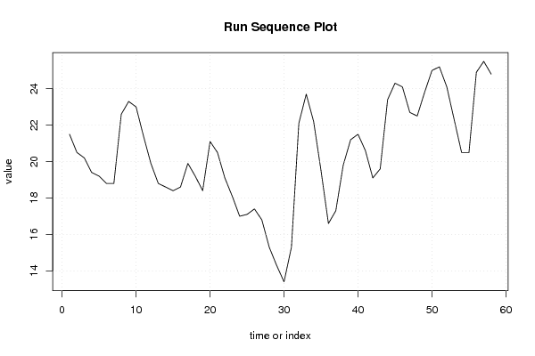
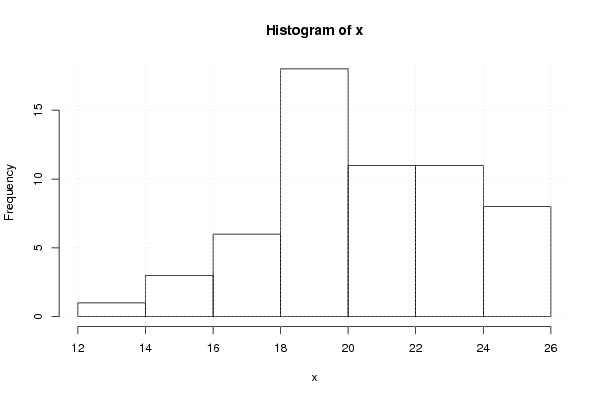
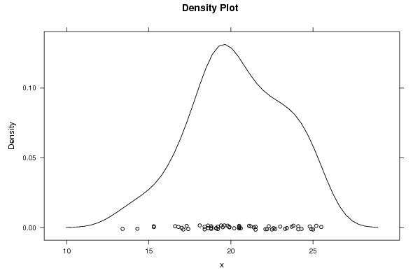
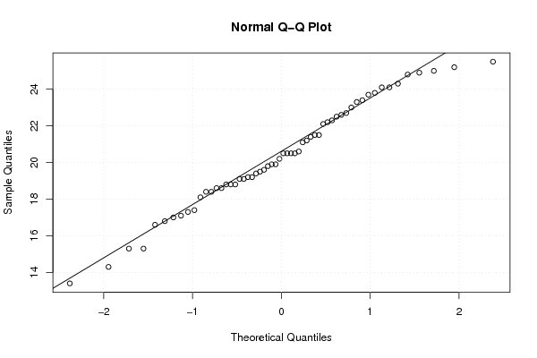
| Dataseries X: | |||||||||||||||||||||||||||||||||||||||||||||||||||||
21.5 20.5 20.2 19.4 19.2 18.8 18.8 22.6 23.3 23 21.4 19.9 18.8 18.6 18.4 18.6 19.9 19.2 18.4 21.1 20.5 19.1 18.1 17 17.1 17.4 16.8 15.3 14.3 13.4 15.3 22.1 23.7 22.2 19.5 16.6 17.3 19.8 21.2 21.5 20.6 19.1 19.6 23.4 24.3 24.1 22.7 22.5 23.8 25 25.2 24.1 22.3 20.5 20.5 24.9 25.5 24.8 | |||||||||||||||||||||||||||||||||||||||||||||||||||||
Tables (Output of Computation) | |||||||||||||||||||||||||||||||||||||||||||||||||||||
| |||||||||||||||||||||||||||||||||||||||||||||||||||||
Figures (Output of Computation) | |||||||||||||||||||||||||||||||||||||||||||||||||||||
Input Parameters & R Code | |||||||||||||||||||||||||||||||||||||||||||||||||||||
| Parameters (Session): | |||||||||||||||||||||||||||||||||||||||||||||||||||||
| par1 = 0 ; par2 = 0 ; | |||||||||||||||||||||||||||||||||||||||||||||||||||||
| Parameters (R input): | |||||||||||||||||||||||||||||||||||||||||||||||||||||
| par1 = 0 ; par2 = 0 ; | |||||||||||||||||||||||||||||||||||||||||||||||||||||
| R code (references can be found in the software module): | |||||||||||||||||||||||||||||||||||||||||||||||||||||
par1 <- as.numeric(par1) | |||||||||||||||||||||||||||||||||||||||||||||||||||||