Repository of Reproducible Computations

Free Statistics

of Irreproducible Research!

Author's title

Author

*The author of this computation has been verified*

R Software Module

rwasp_autocorrelation.wasp

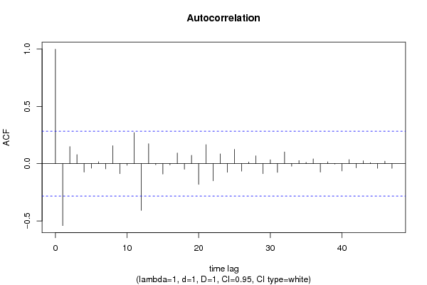
Title produced by software

(Partial) Autocorrelation Function

Date of computation

Thu, 16 Dec 2010 14:18:31 +0000

Cite this page as follows

Statistical Computations at FreeStatistics.org, Office for Research Development and Education, URL https://freestatistics.org/blog/index.php?v=date/2010/Dec/16/t1292509075alhxjan0mnbmk6b.htm/, Retrieved Fri, 03 May 2024 10:43:03 +0000

Statistical Computations at FreeStatistics.org, Office for Research Development and Education, URL https://freestatistics.org/blog/index.php?pk=110954, Retrieved Fri, 03 May 2024 10:43:03 +0000

QR Codes:

Paste this QR Code to cite your computation.

Original text written by user:

IsPrivate?

No (this computation is public)

User-defined keywords

Estimated Impact

146

Family? (F = Feedback message, R = changed R code, M = changed R Module, P = changed Parameters, D = changed Data)

-     [Univariate Data Series] [data set] [2008-12-01 19:54:57] [b98453cac15ba1066b407e146608df68]
- RMP   [(Partial) Autocorrelation Function] [Unemployment] [2010-11-29 09:05:21] [b98453cac15ba1066b407e146608df68]
-   PD    [(Partial) Autocorrelation Function] [] [2010-12-14 13:00:59] [897115520fe7b6114489bc0eeed64548]
-           [(Partial) Autocorrelation Function] [] [2010-12-15 11:02:26] [bfba28641a1925a39268a5d6ad3b00f2]
-    D        [(Partial) Autocorrelation Function] [] [2010-12-16 13:50:41] [94f4aa1c01e87d8321fffb341ed4df07]
-    D          [(Partial) Autocorrelation Function] [] [2010-12-16 14:10:37] [94f4aa1c01e87d8321fffb341ed4df07]
-   P               [(Partial) Autocorrelation Function] [] [2010-12-16 14:18:31] [d1991ab4912b5ede0ff54c26afa5d84c] [Current]
-   P                 [(Partial) Autocorrelation Function] [] [2010-12-16 14:48:03] [94f4aa1c01e87d8321fffb341ed4df07] 

Feedback Forum

Post a new message

Dataseries X:

Download CSV

Histogram

Boxplots

Summary of computational transaction
Raw Input	view raw input (R code)
Raw Output	view raw output of R engine
Computing time	2 seconds
R Server	'RServer@AstonUniversity' @ vre.aston.ac.uk

\begin{tabular}{lllllllll}
\hline
Summary of computational transaction \tabularnewline
Raw Input & view raw input (R code)  \tabularnewline
Raw Output & view raw output of R engine  \tabularnewline
Computing time & 2 seconds \tabularnewline
R Server & 'RServer@AstonUniversity' @ vre.aston.ac.uk \tabularnewline
\hline
\end{tabular}
%Source: https://freestatistics.org/blog/index.php?pk=110954&T=0

[TABLE]
[ROW][C]Summary of computational transaction[/C][/ROW]
[ROW][C]Raw Input[/C][C]view raw input (R code) [/C][/ROW]
[ROW][C]Raw Output[/C][C]view raw output of R engine [/C][/ROW]
[ROW][C]Computing time[/C][C]2 seconds[/C][/ROW]
[ROW][C]R Server[/C][C]'RServer@AstonUniversity' @ vre.aston.ac.uk[/C][/ROW]
[/TABLE]
Source: https://freestatistics.org/blog/index.php?pk=110954&T=0

Globally Unique Identifier (entire table): ba.freestatistics.org/blog/index.php?pk=110954&T=0

As an alternative you can also use a QR Code:

The GUIDs for individual cells are displayed in the table below:

Summary of computational transaction
Raw Input	view raw input (R code)
Raw Output	view raw output of R engine
Computing time	2 seconds
R Server	'RServer@AstonUniversity' @ vre.aston.ac.uk

Autocorrelation Function
Time lag k	ACF(k)	T-STAT	P-value
1	-0.541364	-3.7507	0.000237
2	0.149042	1.0326	0.153484
3	0.078705	0.5453	0.294042
4	-0.073534	-0.5095	0.306383
5	-0.039528	-0.2739	0.392684
6	0.016578	0.1149	0.45452
7	-0.046255	-0.3205	0.375004
8	0.156853	1.0867	0.141296
9	-0.087564	-0.6067	0.273467
10	-0.014466	-0.1002	0.460293
11	0.271007	1.8776	0.03326
12	-0.408874	-2.8328	0.003364
13	0.174186	1.2068	0.116713
14	-0.009705	-0.0672	0.473334
15	-0.090865	-0.6295	0.265992
16	-0.011981	-0.083	0.467097
17	0.09338	0.647	0.260371
18	-0.048649	-0.3371	0.368774
19	0.072198	0.5002	0.309609
20	-0.181216	-1.2555	0.107687
21	0.166441	1.1531	0.127282
22	-0.150442	-1.0423	0.151249
23	0.085689	0.5937	0.27776
24	-0.075989	-0.5265	0.300495
25	0.124741	0.8642	0.19588
26	-0.065335	-0.4527	0.326419
27	0.014318	0.0992	0.460696
28	0.068167	0.4723	0.319436
29	-0.08778	-0.6082	0.272974
30	0.034239	0.2372	0.406751
31	-0.07606	-0.527	0.300324
32	0.101969	0.7065	0.241659
33	-0.022403	-0.1552	0.438653
34	0.026879	0.1862	0.426527
35	0.011297	0.0783	0.468969
36	0.041326	0.2863	0.387934
37	-0.07447	-0.5159	0.304131
38	0.01601	0.1109	0.456072
39	-0.00448	-0.031	0.487684
40	-0.063761	-0.4418	0.330326
41	0.035221	0.244	0.404128
42	-0.036665	-0.254	0.400281
43	0.0249	0.1725	0.431879
44	0.008411	0.0583	0.476886
45	-0.040456	-0.2803	0.390231
46	0.021618	0.1498	0.440786
47	-0.041335	-0.2864	0.387912
48	NA	NA	NA
49	NA	NA	NA
50	NA	NA	NA
51	NA	NA	NA
52	NA	NA	NA
53	NA	NA	NA
54	NA	NA	NA
55	NA	NA	NA
56	NA	NA	NA
57	NA	NA	NA
58	NA	NA	NA
59	NA	NA	NA
60	NA	NA	NA

\begin{tabular}{lllllllll}
\hline
Autocorrelation Function \tabularnewline
Time lag k & ACF(k) & T-STAT & P-value \tabularnewline
1 & -0.541364 & -3.7507 & 0.000237 \tabularnewline
2 & 0.149042 & 1.0326 & 0.153484 \tabularnewline
3 & 0.078705 & 0.5453 & 0.294042 \tabularnewline
4 & -0.073534 & -0.5095 & 0.306383 \tabularnewline
5 & -0.039528 & -0.2739 & 0.392684 \tabularnewline
6 & 0.016578 & 0.1149 & 0.45452 \tabularnewline
7 & -0.046255 & -0.3205 & 0.375004 \tabularnewline
8 & 0.156853 & 1.0867 & 0.141296 \tabularnewline
9 & -0.087564 & -0.6067 & 0.273467 \tabularnewline
10 & -0.014466 & -0.1002 & 0.460293 \tabularnewline
11 & 0.271007 & 1.8776 & 0.03326 \tabularnewline
12 & -0.408874 & -2.8328 & 0.003364 \tabularnewline
13 & 0.174186 & 1.2068 & 0.116713 \tabularnewline
14 & -0.009705 & -0.0672 & 0.473334 \tabularnewline
15 & -0.090865 & -0.6295 & 0.265992 \tabularnewline
16 & -0.011981 & -0.083 & 0.467097 \tabularnewline
17 & 0.09338 & 0.647 & 0.260371 \tabularnewline
18 & -0.048649 & -0.3371 & 0.368774 \tabularnewline
19 & 0.072198 & 0.5002 & 0.309609 \tabularnewline
20 & -0.181216 & -1.2555 & 0.107687 \tabularnewline
21 & 0.166441 & 1.1531 & 0.127282 \tabularnewline
22 & -0.150442 & -1.0423 & 0.151249 \tabularnewline
23 & 0.085689 & 0.5937 & 0.27776 \tabularnewline
24 & -0.075989 & -0.5265 & 0.300495 \tabularnewline
25 & 0.124741 & 0.8642 & 0.19588 \tabularnewline
26 & -0.065335 & -0.4527 & 0.326419 \tabularnewline
27 & 0.014318 & 0.0992 & 0.460696 \tabularnewline
28 & 0.068167 & 0.4723 & 0.319436 \tabularnewline
29 & -0.08778 & -0.6082 & 0.272974 \tabularnewline
30 & 0.034239 & 0.2372 & 0.406751 \tabularnewline
31 & -0.07606 & -0.527 & 0.300324 \tabularnewline
32 & 0.101969 & 0.7065 & 0.241659 \tabularnewline
33 & -0.022403 & -0.1552 & 0.438653 \tabularnewline
34 & 0.026879 & 0.1862 & 0.426527 \tabularnewline
35 & 0.011297 & 0.0783 & 0.468969 \tabularnewline
36 & 0.041326 & 0.2863 & 0.387934 \tabularnewline
37 & -0.07447 & -0.5159 & 0.304131 \tabularnewline
38 & 0.01601 & 0.1109 & 0.456072 \tabularnewline
39 & -0.00448 & -0.031 & 0.487684 \tabularnewline
40 & -0.063761 & -0.4418 & 0.330326 \tabularnewline
41 & 0.035221 & 0.244 & 0.404128 \tabularnewline
42 & -0.036665 & -0.254 & 0.400281 \tabularnewline
43 & 0.0249 & 0.1725 & 0.431879 \tabularnewline
44 & 0.008411 & 0.0583 & 0.476886 \tabularnewline
45 & -0.040456 & -0.2803 & 0.390231 \tabularnewline
46 & 0.021618 & 0.1498 & 0.440786 \tabularnewline
47 & -0.041335 & -0.2864 & 0.387912 \tabularnewline
48 & NA & NA & NA \tabularnewline
49 & NA & NA & NA \tabularnewline
50 & NA & NA & NA \tabularnewline
51 & NA & NA & NA \tabularnewline
52 & NA & NA & NA \tabularnewline
53 & NA & NA & NA \tabularnewline
54 & NA & NA & NA \tabularnewline
55 & NA & NA & NA \tabularnewline
56 & NA & NA & NA \tabularnewline
57 & NA & NA & NA \tabularnewline
58 & NA & NA & NA \tabularnewline
59 & NA & NA & NA \tabularnewline
60 & NA & NA & NA \tabularnewline
\hline
\end{tabular}
%Source: https://freestatistics.org/blog/index.php?pk=110954&T=1

[TABLE]
[ROW][C]Autocorrelation Function[/C][/ROW]
[ROW][C]Time lag k[/C][C]ACF(k)[/C][C]T-STAT[/C][C]P-value[/C][/ROW]
[ROW][C]1[/C][C]-0.541364[/C][C]-3.7507[/C][C]0.000237[/C][/ROW]
[ROW][C]2[/C][C]0.149042[/C][C]1.0326[/C][C]0.153484[/C][/ROW]
[ROW][C]3[/C][C]0.078705[/C][C]0.5453[/C][C]0.294042[/C][/ROW]
[ROW][C]4[/C][C]-0.073534[/C][C]-0.5095[/C][C]0.306383[/C][/ROW]
[ROW][C]5[/C][C]-0.039528[/C][C]-0.2739[/C][C]0.392684[/C][/ROW]
[ROW][C]6[/C][C]0.016578[/C][C]0.1149[/C][C]0.45452[/C][/ROW]
[ROW][C]7[/C][C]-0.046255[/C][C]-0.3205[/C][C]0.375004[/C][/ROW]
[ROW][C]8[/C][C]0.156853[/C][C]1.0867[/C][C]0.141296[/C][/ROW]
[ROW][C]9[/C][C]-0.087564[/C][C]-0.6067[/C][C]0.273467[/C][/ROW]
[ROW][C]10[/C][C]-0.014466[/C][C]-0.1002[/C][C]0.460293[/C][/ROW]
[ROW][C]11[/C][C]0.271007[/C][C]1.8776[/C][C]0.03326[/C][/ROW]
[ROW][C]12[/C][C]-0.408874[/C][C]-2.8328[/C][C]0.003364[/C][/ROW]
[ROW][C]13[/C][C]0.174186[/C][C]1.2068[/C][C]0.116713[/C][/ROW]
[ROW][C]14[/C][C]-0.009705[/C][C]-0.0672[/C][C]0.473334[/C][/ROW]
[ROW][C]15[/C][C]-0.090865[/C][C]-0.6295[/C][C]0.265992[/C][/ROW]
[ROW][C]16[/C][C]-0.011981[/C][C]-0.083[/C][C]0.467097[/C][/ROW]
[ROW][C]17[/C][C]0.09338[/C][C]0.647[/C][C]0.260371[/C][/ROW]
[ROW][C]18[/C][C]-0.048649[/C][C]-0.3371[/C][C]0.368774[/C][/ROW]
[ROW][C]19[/C][C]0.072198[/C][C]0.5002[/C][C]0.309609[/C][/ROW]
[ROW][C]20[/C][C]-0.181216[/C][C]-1.2555[/C][C]0.107687[/C][/ROW]
[ROW][C]21[/C][C]0.166441[/C][C]1.1531[/C][C]0.127282[/C][/ROW]
[ROW][C]22[/C][C]-0.150442[/C][C]-1.0423[/C][C]0.151249[/C][/ROW]
[ROW][C]23[/C][C]0.085689[/C][C]0.5937[/C][C]0.27776[/C][/ROW]
[ROW][C]24[/C][C]-0.075989[/C][C]-0.5265[/C][C]0.300495[/C][/ROW]
[ROW][C]25[/C][C]0.124741[/C][C]0.8642[/C][C]0.19588[/C][/ROW]
[ROW][C]26[/C][C]-0.065335[/C][C]-0.4527[/C][C]0.326419[/C][/ROW]
[ROW][C]27[/C][C]0.014318[/C][C]0.0992[/C][C]0.460696[/C][/ROW]
[ROW][C]28[/C][C]0.068167[/C][C]0.4723[/C][C]0.319436[/C][/ROW]
[ROW][C]29[/C][C]-0.08778[/C][C]-0.6082[/C][C]0.272974[/C][/ROW]
[ROW][C]30[/C][C]0.034239[/C][C]0.2372[/C][C]0.406751[/C][/ROW]
[ROW][C]31[/C][C]-0.07606[/C][C]-0.527[/C][C]0.300324[/C][/ROW]
[ROW][C]32[/C][C]0.101969[/C][C]0.7065[/C][C]0.241659[/C][/ROW]
[ROW][C]33[/C][C]-0.022403[/C][C]-0.1552[/C][C]0.438653[/C][/ROW]
[ROW][C]34[/C][C]0.026879[/C][C]0.1862[/C][C]0.426527[/C][/ROW]
[ROW][C]35[/C][C]0.011297[/C][C]0.0783[/C][C]0.468969[/C][/ROW]
[ROW][C]36[/C][C]0.041326[/C][C]0.2863[/C][C]0.387934[/C][/ROW]
[ROW][C]37[/C][C]-0.07447[/C][C]-0.5159[/C][C]0.304131[/C][/ROW]
[ROW][C]38[/C][C]0.01601[/C][C]0.1109[/C][C]0.456072[/C][/ROW]
[ROW][C]39[/C][C]-0.00448[/C][C]-0.031[/C][C]0.487684[/C][/ROW]
[ROW][C]40[/C][C]-0.063761[/C][C]-0.4418[/C][C]0.330326[/C][/ROW]
[ROW][C]41[/C][C]0.035221[/C][C]0.244[/C][C]0.404128[/C][/ROW]
[ROW][C]42[/C][C]-0.036665[/C][C]-0.254[/C][C]0.400281[/C][/ROW]
[ROW][C]43[/C][C]0.0249[/C][C]0.1725[/C][C]0.431879[/C][/ROW]
[ROW][C]44[/C][C]0.008411[/C][C]0.0583[/C][C]0.476886[/C][/ROW]
[ROW][C]45[/C][C]-0.040456[/C][C]-0.2803[/C][C]0.390231[/C][/ROW]
[ROW][C]46[/C][C]0.021618[/C][C]0.1498[/C][C]0.440786[/C][/ROW]
[ROW][C]47[/C][C]-0.041335[/C][C]-0.2864[/C][C]0.387912[/C][/ROW]
[ROW][C]48[/C][C]NA[/C][C]NA[/C][C]NA[/C][/ROW]
[ROW][C]49[/C][C]NA[/C][C]NA[/C][C]NA[/C][/ROW]
[ROW][C]50[/C][C]NA[/C][C]NA[/C][C]NA[/C][/ROW]
[ROW][C]51[/C][C]NA[/C][C]NA[/C][C]NA[/C][/ROW]
[ROW][C]52[/C][C]NA[/C][C]NA[/C][C]NA[/C][/ROW]
[ROW][C]53[/C][C]NA[/C][C]NA[/C][C]NA[/C][/ROW]
[ROW][C]54[/C][C]NA[/C][C]NA[/C][C]NA[/C][/ROW]
[ROW][C]55[/C][C]NA[/C][C]NA[/C][C]NA[/C][/ROW]
[ROW][C]56[/C][C]NA[/C][C]NA[/C][C]NA[/C][/ROW]
[ROW][C]57[/C][C]NA[/C][C]NA[/C][C]NA[/C][/ROW]
[ROW][C]58[/C][C]NA[/C][C]NA[/C][C]NA[/C][/ROW]
[ROW][C]59[/C][C]NA[/C][C]NA[/C][C]NA[/C][/ROW]
[ROW][C]60[/C][C]NA[/C][C]NA[/C][C]NA[/C][/ROW]
[/TABLE]
Source: https://freestatistics.org/blog/index.php?pk=110954&T=1

Globally Unique Identifier (entire table): ba.freestatistics.org/blog/index.php?pk=110954&T=1

As an alternative you can also use a QR Code:

The GUIDs for individual cells are displayed in the table below:

Autocorrelation Function
Time lag k	ACF(k)	T-STAT	P-value
1	-0.541364	-3.7507	0.000237
2	0.149042	1.0326	0.153484
3	0.078705	0.5453	0.294042
4	-0.073534	-0.5095	0.306383
5	-0.039528	-0.2739	0.392684
6	0.016578	0.1149	0.45452
7	-0.046255	-0.3205	0.375004
8	0.156853	1.0867	0.141296
9	-0.087564	-0.6067	0.273467
10	-0.014466	-0.1002	0.460293
11	0.271007	1.8776	0.03326
12	-0.408874	-2.8328	0.003364
13	0.174186	1.2068	0.116713
14	-0.009705	-0.0672	0.473334
15	-0.090865	-0.6295	0.265992
16	-0.011981	-0.083	0.467097
17	0.09338	0.647	0.260371
18	-0.048649	-0.3371	0.368774
19	0.072198	0.5002	0.309609
20	-0.181216	-1.2555	0.107687
21	0.166441	1.1531	0.127282
22	-0.150442	-1.0423	0.151249
23	0.085689	0.5937	0.27776
24	-0.075989	-0.5265	0.300495
25	0.124741	0.8642	0.19588
26	-0.065335	-0.4527	0.326419
27	0.014318	0.0992	0.460696
28	0.068167	0.4723	0.319436
29	-0.08778	-0.6082	0.272974
30	0.034239	0.2372	0.406751
31	-0.07606	-0.527	0.300324
32	0.101969	0.7065	0.241659
33	-0.022403	-0.1552	0.438653
34	0.026879	0.1862	0.426527
35	0.011297	0.0783	0.468969
36	0.041326	0.2863	0.387934
37	-0.07447	-0.5159	0.304131
38	0.01601	0.1109	0.456072
39	-0.00448	-0.031	0.487684
40	-0.063761	-0.4418	0.330326
41	0.035221	0.244	0.404128
42	-0.036665	-0.254	0.400281
43	0.0249	0.1725	0.431879
44	0.008411	0.0583	0.476886
45	-0.040456	-0.2803	0.390231
46	0.021618	0.1498	0.440786
47	-0.041335	-0.2864	0.387912
48	NA	NA	NA
49	NA	NA	NA
50	NA	NA	NA
51	NA	NA	NA
52	NA	NA	NA
53	NA	NA	NA
54	NA	NA	NA
55	NA	NA	NA
56	NA	NA	NA
57	NA	NA	NA
58	NA	NA	NA
59	NA	NA	NA
60	NA	NA	NA

Partial Autocorrelation Function
Time lag k	PACF(k)	T-STAT	P-value
1	-0.541364	-3.7507	0.000237
2	-0.203745	-1.4116	0.082261
3	0.096713	0.67	0.25302
4	0.073795	0.5113	0.305753
5	-0.086401	-0.5986	0.276126
6	-0.116276	-0.8056	0.212228
7	-0.105289	-0.7295	0.234631
8	0.18575	1.2869	0.102147
9	0.162159	1.1235	0.133413
10	-0.045811	-0.3174	0.376162
11	0.256553	1.7775	0.040915
12	-0.189036	-1.3097	0.098269
13	-0.228834	-1.5854	0.05972
14	-0.058444	-0.4049	0.343671
15	0.019121	0.1325	0.447581
16	-0.083582	-0.5791	0.282623
17	-0.016954	-0.1175	0.453494
18	-0.001786	-0.0124	0.495088
19	0.010711	0.0742	0.470576
20	-0.149256	-1.0341	0.153142
21	0.001403	0.0097	0.496141
22	-0.121994	-0.8452	0.201097
23	0.245732	1.7025	0.047567
24	-0.019414	-0.1345	0.446784
25	0.010089	0.0699	0.472283
26	0.040524	0.2808	0.39005
27	-0.02866	-0.1986	0.421721
28	0.022465	0.1556	0.438483
29	-0.003205	-0.0222	0.491187
30	0.046065	0.3191	0.3755
31	-0.084726	-0.587	0.279977
32	-0.086641	-0.6003	0.275576
33	0.139814	0.9687	0.168786
34	-0.007017	-0.0486	0.480714
35	0.133123	0.9223	0.180491
36	-0.069176	-0.4793	0.316963
37	-0.029857	-0.2069	0.418499
38	0.002724	0.0189	0.492511
39	-0.007985	-0.0553	0.478057
40	-0.072649	-0.5033	0.308518
41	-0.059723	-0.4138	0.340441
42	-0.100692	-0.6976	0.244392
43	-0.098461	-0.6822	0.24921
44	-0.080632	-0.5586	0.289504
45	0.11463	0.7942	0.2155
46	-0.086464	-0.599	0.275981
47	0.009858	0.0683	0.472916
48	NA	NA	NA
49	NA	NA	NA
50	NA	NA	NA
51	NA	NA	NA
52	NA	NA	NA
53	NA	NA	NA
54	NA	NA	NA
55	NA	NA	NA
56	NA	NA	NA
57	NA	NA	NA
58	NA	NA	NA
59	NA	NA	NA
60	NA	NA	NA

\begin{tabular}{lllllllll}
\hline
Partial Autocorrelation Function \tabularnewline
Time lag k & PACF(k) & T-STAT & P-value \tabularnewline
1 & -0.541364 & -3.7507 & 0.000237 \tabularnewline
2 & -0.203745 & -1.4116 & 0.082261 \tabularnewline
3 & 0.096713 & 0.67 & 0.25302 \tabularnewline
4 & 0.073795 & 0.5113 & 0.305753 \tabularnewline
5 & -0.086401 & -0.5986 & 0.276126 \tabularnewline
6 & -0.116276 & -0.8056 & 0.212228 \tabularnewline
7 & -0.105289 & -0.7295 & 0.234631 \tabularnewline
8 & 0.18575 & 1.2869 & 0.102147 \tabularnewline
9 & 0.162159 & 1.1235 & 0.133413 \tabularnewline
10 & -0.045811 & -0.3174 & 0.376162 \tabularnewline
11 & 0.256553 & 1.7775 & 0.040915 \tabularnewline
12 & -0.189036 & -1.3097 & 0.098269 \tabularnewline
13 & -0.228834 & -1.5854 & 0.05972 \tabularnewline
14 & -0.058444 & -0.4049 & 0.343671 \tabularnewline
15 & 0.019121 & 0.1325 & 0.447581 \tabularnewline
16 & -0.083582 & -0.5791 & 0.282623 \tabularnewline
17 & -0.016954 & -0.1175 & 0.453494 \tabularnewline
18 & -0.001786 & -0.0124 & 0.495088 \tabularnewline
19 & 0.010711 & 0.0742 & 0.470576 \tabularnewline
20 & -0.149256 & -1.0341 & 0.153142 \tabularnewline
21 & 0.001403 & 0.0097 & 0.496141 \tabularnewline
22 & -0.121994 & -0.8452 & 0.201097 \tabularnewline
23 & 0.245732 & 1.7025 & 0.047567 \tabularnewline
24 & -0.019414 & -0.1345 & 0.446784 \tabularnewline
25 & 0.010089 & 0.0699 & 0.472283 \tabularnewline
26 & 0.040524 & 0.2808 & 0.39005 \tabularnewline
27 & -0.02866 & -0.1986 & 0.421721 \tabularnewline
28 & 0.022465 & 0.1556 & 0.438483 \tabularnewline
29 & -0.003205 & -0.0222 & 0.491187 \tabularnewline
30 & 0.046065 & 0.3191 & 0.3755 \tabularnewline
31 & -0.084726 & -0.587 & 0.279977 \tabularnewline
32 & -0.086641 & -0.6003 & 0.275576 \tabularnewline
33 & 0.139814 & 0.9687 & 0.168786 \tabularnewline
34 & -0.007017 & -0.0486 & 0.480714 \tabularnewline
35 & 0.133123 & 0.9223 & 0.180491 \tabularnewline
36 & -0.069176 & -0.4793 & 0.316963 \tabularnewline
37 & -0.029857 & -0.2069 & 0.418499 \tabularnewline
38 & 0.002724 & 0.0189 & 0.492511 \tabularnewline
39 & -0.007985 & -0.0553 & 0.478057 \tabularnewline
40 & -0.072649 & -0.5033 & 0.308518 \tabularnewline
41 & -0.059723 & -0.4138 & 0.340441 \tabularnewline
42 & -0.100692 & -0.6976 & 0.244392 \tabularnewline
43 & -0.098461 & -0.6822 & 0.24921 \tabularnewline
44 & -0.080632 & -0.5586 & 0.289504 \tabularnewline
45 & 0.11463 & 0.7942 & 0.2155 \tabularnewline
46 & -0.086464 & -0.599 & 0.275981 \tabularnewline
47 & 0.009858 & 0.0683 & 0.472916 \tabularnewline
48 & NA & NA & NA \tabularnewline
49 & NA & NA & NA \tabularnewline
50 & NA & NA & NA \tabularnewline
51 & NA & NA & NA \tabularnewline
52 & NA & NA & NA \tabularnewline
53 & NA & NA & NA \tabularnewline
54 & NA & NA & NA \tabularnewline
55 & NA & NA & NA \tabularnewline
56 & NA & NA & NA \tabularnewline
57 & NA & NA & NA \tabularnewline
58 & NA & NA & NA \tabularnewline
59 & NA & NA & NA \tabularnewline
60 & NA & NA & NA \tabularnewline
\hline
\end{tabular}
%Source: https://freestatistics.org/blog/index.php?pk=110954&T=2

[TABLE]
[ROW][C]Partial Autocorrelation Function[/C][/ROW]
[ROW][C]Time lag k[/C][C]PACF(k)[/C][C]T-STAT[/C][C]P-value[/C][/ROW]
[ROW][C]1[/C][C]-0.541364[/C][C]-3.7507[/C][C]0.000237[/C][/ROW]
[ROW][C]2[/C][C]-0.203745[/C][C]-1.4116[/C][C]0.082261[/C][/ROW]
[ROW][C]3[/C][C]0.096713[/C][C]0.67[/C][C]0.25302[/C][/ROW]
[ROW][C]4[/C][C]0.073795[/C][C]0.5113[/C][C]0.305753[/C][/ROW]
[ROW][C]5[/C][C]-0.086401[/C][C]-0.5986[/C][C]0.276126[/C][/ROW]
[ROW][C]6[/C][C]-0.116276[/C][C]-0.8056[/C][C]0.212228[/C][/ROW]
[ROW][C]7[/C][C]-0.105289[/C][C]-0.7295[/C][C]0.234631[/C][/ROW]
[ROW][C]8[/C][C]0.18575[/C][C]1.2869[/C][C]0.102147[/C][/ROW]
[ROW][C]9[/C][C]0.162159[/C][C]1.1235[/C][C]0.133413[/C][/ROW]
[ROW][C]10[/C][C]-0.045811[/C][C]-0.3174[/C][C]0.376162[/C][/ROW]
[ROW][C]11[/C][C]0.256553[/C][C]1.7775[/C][C]0.040915[/C][/ROW]
[ROW][C]12[/C][C]-0.189036[/C][C]-1.3097[/C][C]0.098269[/C][/ROW]
[ROW][C]13[/C][C]-0.228834[/C][C]-1.5854[/C][C]0.05972[/C][/ROW]
[ROW][C]14[/C][C]-0.058444[/C][C]-0.4049[/C][C]0.343671[/C][/ROW]
[ROW][C]15[/C][C]0.019121[/C][C]0.1325[/C][C]0.447581[/C][/ROW]
[ROW][C]16[/C][C]-0.083582[/C][C]-0.5791[/C][C]0.282623[/C][/ROW]
[ROW][C]17[/C][C]-0.016954[/C][C]-0.1175[/C][C]0.453494[/C][/ROW]
[ROW][C]18[/C][C]-0.001786[/C][C]-0.0124[/C][C]0.495088[/C][/ROW]
[ROW][C]19[/C][C]0.010711[/C][C]0.0742[/C][C]0.470576[/C][/ROW]
[ROW][C]20[/C][C]-0.149256[/C][C]-1.0341[/C][C]0.153142[/C][/ROW]
[ROW][C]21[/C][C]0.001403[/C][C]0.0097[/C][C]0.496141[/C][/ROW]
[ROW][C]22[/C][C]-0.121994[/C][C]-0.8452[/C][C]0.201097[/C][/ROW]
[ROW][C]23[/C][C]0.245732[/C][C]1.7025[/C][C]0.047567[/C][/ROW]
[ROW][C]24[/C][C]-0.019414[/C][C]-0.1345[/C][C]0.446784[/C][/ROW]
[ROW][C]25[/C][C]0.010089[/C][C]0.0699[/C][C]0.472283[/C][/ROW]
[ROW][C]26[/C][C]0.040524[/C][C]0.2808[/C][C]0.39005[/C][/ROW]
[ROW][C]27[/C][C]-0.02866[/C][C]-0.1986[/C][C]0.421721[/C][/ROW]
[ROW][C]28[/C][C]0.022465[/C][C]0.1556[/C][C]0.438483[/C][/ROW]
[ROW][C]29[/C][C]-0.003205[/C][C]-0.0222[/C][C]0.491187[/C][/ROW]
[ROW][C]30[/C][C]0.046065[/C][C]0.3191[/C][C]0.3755[/C][/ROW]
[ROW][C]31[/C][C]-0.084726[/C][C]-0.587[/C][C]0.279977[/C][/ROW]
[ROW][C]32[/C][C]-0.086641[/C][C]-0.6003[/C][C]0.275576[/C][/ROW]
[ROW][C]33[/C][C]0.139814[/C][C]0.9687[/C][C]0.168786[/C][/ROW]
[ROW][C]34[/C][C]-0.007017[/C][C]-0.0486[/C][C]0.480714[/C][/ROW]
[ROW][C]35[/C][C]0.133123[/C][C]0.9223[/C][C]0.180491[/C][/ROW]
[ROW][C]36[/C][C]-0.069176[/C][C]-0.4793[/C][C]0.316963[/C][/ROW]
[ROW][C]37[/C][C]-0.029857[/C][C]-0.2069[/C][C]0.418499[/C][/ROW]
[ROW][C]38[/C][C]0.002724[/C][C]0.0189[/C][C]0.492511[/C][/ROW]
[ROW][C]39[/C][C]-0.007985[/C][C]-0.0553[/C][C]0.478057[/C][/ROW]
[ROW][C]40[/C][C]-0.072649[/C][C]-0.5033[/C][C]0.308518[/C][/ROW]
[ROW][C]41[/C][C]-0.059723[/C][C]-0.4138[/C][C]0.340441[/C][/ROW]
[ROW][C]42[/C][C]-0.100692[/C][C]-0.6976[/C][C]0.244392[/C][/ROW]
[ROW][C]43[/C][C]-0.098461[/C][C]-0.6822[/C][C]0.24921[/C][/ROW]
[ROW][C]44[/C][C]-0.080632[/C][C]-0.5586[/C][C]0.289504[/C][/ROW]
[ROW][C]45[/C][C]0.11463[/C][C]0.7942[/C][C]0.2155[/C][/ROW]
[ROW][C]46[/C][C]-0.086464[/C][C]-0.599[/C][C]0.275981[/C][/ROW]
[ROW][C]47[/C][C]0.009858[/C][C]0.0683[/C][C]0.472916[/C][/ROW]
[ROW][C]48[/C][C]NA[/C][C]NA[/C][C]NA[/C][/ROW]
[ROW][C]49[/C][C]NA[/C][C]NA[/C][C]NA[/C][/ROW]
[ROW][C]50[/C][C]NA[/C][C]NA[/C][C]NA[/C][/ROW]
[ROW][C]51[/C][C]NA[/C][C]NA[/C][C]NA[/C][/ROW]
[ROW][C]52[/C][C]NA[/C][C]NA[/C][C]NA[/C][/ROW]
[ROW][C]53[/C][C]NA[/C][C]NA[/C][C]NA[/C][/ROW]
[ROW][C]54[/C][C]NA[/C][C]NA[/C][C]NA[/C][/ROW]
[ROW][C]55[/C][C]NA[/C][C]NA[/C][C]NA[/C][/ROW]
[ROW][C]56[/C][C]NA[/C][C]NA[/C][C]NA[/C][/ROW]
[ROW][C]57[/C][C]NA[/C][C]NA[/C][C]NA[/C][/ROW]
[ROW][C]58[/C][C]NA[/C][C]NA[/C][C]NA[/C][/ROW]
[ROW][C]59[/C][C]NA[/C][C]NA[/C][C]NA[/C][/ROW]
[ROW][C]60[/C][C]NA[/C][C]NA[/C][C]NA[/C][/ROW]
[/TABLE]
Source: https://freestatistics.org/blog/index.php?pk=110954&T=2

Globally Unique Identifier (entire table): ba.freestatistics.org/blog/index.php?pk=110954&T=2

As an alternative you can also use a QR Code:

The GUIDs for individual cells are displayed in the table below:

Partial Autocorrelation Function
Time lag k	PACF(k)	T-STAT	P-value
1	-0.541364	-3.7507	0.000237
2	-0.203745	-1.4116	0.082261
3	0.096713	0.67	0.25302
4	0.073795	0.5113	0.305753
5	-0.086401	-0.5986	0.276126
6	-0.116276	-0.8056	0.212228
7	-0.105289	-0.7295	0.234631
8	0.18575	1.2869	0.102147
9	0.162159	1.1235	0.133413
10	-0.045811	-0.3174	0.376162
11	0.256553	1.7775	0.040915
12	-0.189036	-1.3097	0.098269
13	-0.228834	-1.5854	0.05972
14	-0.058444	-0.4049	0.343671
15	0.019121	0.1325	0.447581
16	-0.083582	-0.5791	0.282623
17	-0.016954	-0.1175	0.453494
18	-0.001786	-0.0124	0.495088
19	0.010711	0.0742	0.470576
20	-0.149256	-1.0341	0.153142
21	0.001403	0.0097	0.496141
22	-0.121994	-0.8452	0.201097
23	0.245732	1.7025	0.047567
24	-0.019414	-0.1345	0.446784
25	0.010089	0.0699	0.472283
26	0.040524	0.2808	0.39005
27	-0.02866	-0.1986	0.421721
28	0.022465	0.1556	0.438483
29	-0.003205	-0.0222	0.491187
30	0.046065	0.3191	0.3755
31	-0.084726	-0.587	0.279977
32	-0.086641	-0.6003	0.275576
33	0.139814	0.9687	0.168786
34	-0.007017	-0.0486	0.480714
35	0.133123	0.9223	0.180491
36	-0.069176	-0.4793	0.316963
37	-0.029857	-0.2069	0.418499
38	0.002724	0.0189	0.492511
39	-0.007985	-0.0553	0.478057
40	-0.072649	-0.5033	0.308518
41	-0.059723	-0.4138	0.340441
42	-0.100692	-0.6976	0.244392
43	-0.098461	-0.6822	0.24921
44	-0.080632	-0.5586	0.289504
45	0.11463	0.7942	0.2155
46	-0.086464	-0.599	0.275981
47	0.009858	0.0683	0.472916
48	NA	NA	NA
49	NA	NA	NA
50	NA	NA	NA
51	NA	NA	NA
52	NA	NA	NA
53	NA	NA	NA
54	NA	NA	NA
55	NA	NA	NA
56	NA	NA	NA
57	NA	NA	NA
58	NA	NA	NA
59	NA	NA	NA
60	NA	NA	NA

Figure 1

PNG link

Postscript link

PDF link

Figure 2

PNG link

Postscript link

PDF link

Parameters (Session):

par1 = 60 ; par2 = 1 ; par3 = 1 ; par4 = 1 ; par5 = 12 ; par6 = White Noise ; par7 = 0.95 ;

Parameters (R input):

par1 = 60 ; par2 = 1 ; par3 = 1 ; par4 = 1 ; par5 = 12 ; par6 = White Noise ; par7 = 0.95 ; par8 = ;

R code (references can be found in the software module):

if (par1 == 'Default') {
par1 = 10*log10(length(x))
} else {
par1 <- as.numeric(par1)
}
par2 <- as.numeric(par2)
par3 <- as.numeric(par3)
par4 <- as.numeric(par4)
par5 <- as.numeric(par5)
if (par6 == 'White Noise') par6 <- 'white' else par6 <- 'ma'
par7 <- as.numeric(par7)
if (par2 == 0) {
x <- log(x)
} else {
x <- (x ^ par2 - 1) / par2
}
if (par3 > 0) x <- diff(x,lag=1,difference=par3)
if (par4 > 0) x <- diff(x,lag=par5,difference=par4)
bitmap(file='pic1.png')
racf <- acf(x, par1, main='Autocorrelation', xlab='time lag', ylab='ACF', ci.type=par6, ci=par7, sub=paste('(lambda=',par2,', d=',par3,', D=',par4,', CI=', par7, ', CI type=',par6,')',sep=''))
dev.off()
bitmap(file='pic2.png')
rpacf <- pacf(x,par1,main='Partial Autocorrelation',xlab='lags',ylab='PACF')
dev.off()
(myacf <- c(racf$acf))
(mypacf <- c(rpacf$acf))
lengthx <- length(x)
sqrtn <- sqrt(lengthx)
load(file='createtable')
a<-table.start()
a<-table.row.start(a)
a<-table.element(a,'Autocorrelation Function',4,TRUE)
a<-table.row.end(a)
a<-table.row.start(a)
a<-table.element(a,'Time lag k',header=TRUE)
a<-table.element(a,hyperlink('basics.htm','ACF(k)','click here for more information about the Autocorrelation Function'),header=TRUE)
a<-table.element(a,'T-STAT',header=TRUE)
a<-table.element(a,'P-value',header=TRUE)
a<-table.row.end(a)
for (i in 2:(par1+1)) {
a<-table.row.start(a)
a<-table.element(a,i-1,header=TRUE)
a<-table.element(a,round(myacf[i],6))
mytstat <- myacf[i]*sqrtn
a<-table.element(a,round(mytstat,4))
a<-table.element(a,round(1-pt(abs(mytstat),lengthx),6))
a<-table.row.end(a)
}
a<-table.end(a)
table.save(a,file='mytable.tab')
a<-table.start()
a<-table.row.start(a)
a<-table.element(a,'Partial Autocorrelation Function',4,TRUE)
a<-table.row.end(a)
a<-table.row.start(a)
a<-table.element(a,'Time lag k',header=TRUE)
a<-table.element(a,hyperlink('basics.htm','PACF(k)','click here for more information about the Partial Autocorrelation Function'),header=TRUE)
a<-table.element(a,'T-STAT',header=TRUE)
a<-table.element(a,'P-value',header=TRUE)
a<-table.row.end(a)
for (i in 1:par1) {
a<-table.row.start(a)
a<-table.element(a,i,header=TRUE)
a<-table.element(a,round(mypacf[i],6))
mytstat <- mypacf[i]*sqrtn
a<-table.element(a,round(mytstat,4))
a<-table.element(a,round(1-pt(abs(mytstat),lengthx),6))
a<-table.row.end(a)
}
a<-table.end(a)
table.save(a,file='mytable1.tab')

Free Statistics

Description of Statistical Computation

Tree of Dependent Computations

Dataset

Tables (Output of Computation)

Figures (Output of Computation)

Input Parameters & R Code