Repository of Reproducible Computations

Free Statistics

of Irreproducible Research!

Author's title

Author

*The author of this computation has been verified*

R Software Module

rwasp_arimaforecasting.wasp

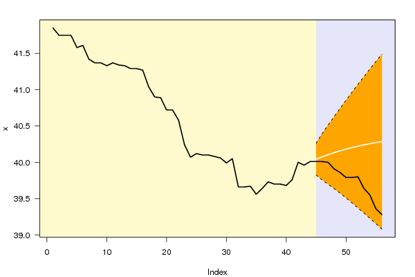
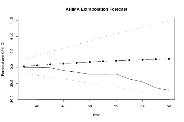
Title produced by software

ARIMA Forecasting

Date of computation

Thu, 16 Dec 2010 10:48:12 +0000

Cite this page as follows

Statistical Computations at FreeStatistics.org, Office for Research Development and Education, URL https://freestatistics.org/blog/index.php?v=date/2010/Dec/16/t1292496375ery7585d7oshwxn.htm/, Retrieved Fri, 03 May 2024 12:09:09 +0000

Statistical Computations at FreeStatistics.org, Office for Research Development and Education, URL https://freestatistics.org/blog/index.php?pk=110848, Retrieved Fri, 03 May 2024 12:09:09 +0000

QR Codes:

Paste this QR Code to cite your computation.

Original text written by user:

IsPrivate?

No (this computation is public)

User-defined keywords

Estimated Impact

150

Family? (F = Feedback message, R = changed R code, M = changed R Module, P = changed Parameters, D = changed Data)

-     [Univariate Data Series] [] [2008-12-08 19:22:39] [d2d412c7f4d35ffbf5ee5ee89db327d4]
- RMP   [Spectral Analysis] [spectrum analyse ...] [2010-12-14 18:46:58] [d6e648f00513dd750579ba7880c5fbf5]
- RMP     [ARIMA Forecasting] [arima forecast] [2010-12-14 19:31:52] [d6e648f00513dd750579ba7880c5fbf5]
- R PD        [ARIMA Forecasting] [] [2010-12-16 10:48:12] [7674ee8f347756742f81ca2ada5c384c] [Current]
-   P           [ARIMA Forecasting] [] [2010-12-16 19:09:06] [b10d6b9682dfaaa479f495240bcd67cf] 
-   PD            [ARIMA Forecasting] [] [2010-12-19 15:52:35] [b10d6b9682dfaaa479f495240bcd67cf] 
-    D              [ARIMA Forecasting] [] [2010-12-28 21:16:29] [58af523ef9b33032fd2497c80088399b] 
-   PD                [ARIMA Forecasting] [] [2010-12-29 09:52:04] [126c9e58bb659a0bfb4675d843c2c69e] 
-    D            [ARIMA Forecasting] [] [2010-12-28 20:15:13] [58af523ef9b33032fd2497c80088399b] 
-    D              [ARIMA Forecasting] [] [2010-12-29 09:36:05] [126c9e58bb659a0bfb4675d843c2c69e] 

Feedback Forum

Post a new message

Dataseries X:

Download CSV

Histogram

Boxplots

Summary of computational transaction
Raw Input	view raw input (R code)
Raw Output	view raw output of R engine
Computing time	1 seconds
R Server	'Gwilym Jenkins' @ 72.249.127.135

\begin{tabular}{lllllllll}
\hline
Summary of computational transaction \tabularnewline
Raw Input & view raw input (R code)  \tabularnewline
Raw Output & view raw output of R engine  \tabularnewline
Computing time & 1 seconds \tabularnewline
R Server & 'Gwilym Jenkins' @ 72.249.127.135 \tabularnewline
\hline
\end{tabular}
%Source: https://freestatistics.org/blog/index.php?pk=110848&T=0

[TABLE]
[ROW][C]Summary of computational transaction[/C][/ROW]
[ROW][C]Raw Input[/C][C]view raw input (R code) [/C][/ROW]
[ROW][C]Raw Output[/C][C]view raw output of R engine [/C][/ROW]
[ROW][C]Computing time[/C][C]1 seconds[/C][/ROW]
[ROW][C]R Server[/C][C]'Gwilym Jenkins' @ 72.249.127.135[/C][/ROW]
[/TABLE]
Source: https://freestatistics.org/blog/index.php?pk=110848&T=0

Globally Unique Identifier (entire table): ba.freestatistics.org/blog/index.php?pk=110848&T=0

As an alternative you can also use a QR Code:

The GUIDs for individual cells are displayed in the table below:

Summary of computational transaction
Raw Input	view raw input (R code)
Raw Output	view raw output of R engine
Computing time	1 seconds
R Server	'Gwilym Jenkins' @ 72.249.127.135

Univariate ARIMA Extrapolation Forecast
time	Y[t]	F[t]	95% LB	95% UB	p-value(H0: Y[t] = F[t])	P(F[t]>Y[t-1])	P(F[t]>Y[t-s])	P(F[t]>Y[44])
43	39.96	-	-	-	-	-	-	-
44	40.01	-	-	-	-	-	-	-
45	40.01	40.0433	39.8251	40.2615	0.3824	0.6176	0.6176	0.6176
46	40.01	40.0753	39.7563	40.3943	0.3442	0.6558	0.6558	0.6558
47	40	40.1054	39.6976	40.5132	0.3063	0.6767	0.6767	0.6767
48	39.91	40.1331	39.6376	40.6286	0.1887	0.7008	0.7008	0.6869
49	39.86	40.1586	39.5747	40.7425	0.1581	0.798	0.798	0.691
50	39.79	40.1818	39.5088	40.8549	0.1269	0.8257	0.8257	0.6916
51	39.79	40.2031	39.4406	40.9656	0.1441	0.8559	0.8559	0.6902
52	39.8	40.2226	39.3706	41.0746	0.1655	0.8402	0.8402	0.6876
53	39.64	40.2404	39.2992	41.1815	0.1056	0.8204	0.8204	0.6843
54	39.55	40.2566	39.2268	41.2864	0.0893	0.8797	0.8797	0.6806
55	39.36	40.2715	39.1537	41.3892	0.055	0.8971	0.8971	0.6767
56	39.28	40.285	39.0802	41.4899	0.051	0.9338	0.9338	0.6727

\begin{tabular}{lllllllll}
\hline
Univariate ARIMA Extrapolation Forecast \tabularnewline
time & Y[t] & F[t] & 95% LB & 95% UB & p-value(H0: Y[t] = F[t]) & P(F[t]>Y[t-1]) & P(F[t]>Y[t-s]) & P(F[t]>Y[44]) \tabularnewline
43 & 39.96 & - & - & - & - & - & - & - \tabularnewline
44 & 40.01 & - & - & - & - & - & - & - \tabularnewline
45 & 40.01 & 40.0433 & 39.8251 & 40.2615 & 0.3824 & 0.6176 & 0.6176 & 0.6176 \tabularnewline
46 & 40.01 & 40.0753 & 39.7563 & 40.3943 & 0.3442 & 0.6558 & 0.6558 & 0.6558 \tabularnewline
47 & 40 & 40.1054 & 39.6976 & 40.5132 & 0.3063 & 0.6767 & 0.6767 & 0.6767 \tabularnewline
48 & 39.91 & 40.1331 & 39.6376 & 40.6286 & 0.1887 & 0.7008 & 0.7008 & 0.6869 \tabularnewline
49 & 39.86 & 40.1586 & 39.5747 & 40.7425 & 0.1581 & 0.798 & 0.798 & 0.691 \tabularnewline
50 & 39.79 & 40.1818 & 39.5088 & 40.8549 & 0.1269 & 0.8257 & 0.8257 & 0.6916 \tabularnewline
51 & 39.79 & 40.2031 & 39.4406 & 40.9656 & 0.1441 & 0.8559 & 0.8559 & 0.6902 \tabularnewline
52 & 39.8 & 40.2226 & 39.3706 & 41.0746 & 0.1655 & 0.8402 & 0.8402 & 0.6876 \tabularnewline
53 & 39.64 & 40.2404 & 39.2992 & 41.1815 & 0.1056 & 0.8204 & 0.8204 & 0.6843 \tabularnewline
54 & 39.55 & 40.2566 & 39.2268 & 41.2864 & 0.0893 & 0.8797 & 0.8797 & 0.6806 \tabularnewline
55 & 39.36 & 40.2715 & 39.1537 & 41.3892 & 0.055 & 0.8971 & 0.8971 & 0.6767 \tabularnewline
56 & 39.28 & 40.285 & 39.0802 & 41.4899 & 0.051 & 0.9338 & 0.9338 & 0.6727 \tabularnewline
\hline
\end{tabular}
%Source: https://freestatistics.org/blog/index.php?pk=110848&T=1

[TABLE]
[ROW][C]Univariate ARIMA Extrapolation Forecast[/C][/ROW]
[ROW][C]time[/C][C]Y[t][/C][C]F[t][/C][C]95% LB[/C][C]95% UB[/C][C]p-value(H0: Y[t] = F[t])[/C][C]P(F[t]>Y[t-1])[/C][C]P(F[t]>Y[t-s])[/C][C]P(F[t]>Y[44])[/C][/ROW]
[ROW][C]43[/C][C]39.96[/C][C]-[/C][C]-[/C][C]-[/C][C]-[/C][C]-[/C][C]-[/C][C]-[/C][/ROW]
[ROW][C]44[/C][C]40.01[/C][C]-[/C][C]-[/C][C]-[/C][C]-[/C][C]-[/C][C]-[/C][C]-[/C][/ROW]
[ROW][C]45[/C][C]40.01[/C][C]40.0433[/C][C]39.8251[/C][C]40.2615[/C][C]0.3824[/C][C]0.6176[/C][C]0.6176[/C][C]0.6176[/C][/ROW]
[ROW][C]46[/C][C]40.01[/C][C]40.0753[/C][C]39.7563[/C][C]40.3943[/C][C]0.3442[/C][C]0.6558[/C][C]0.6558[/C][C]0.6558[/C][/ROW]
[ROW][C]47[/C][C]40[/C][C]40.1054[/C][C]39.6976[/C][C]40.5132[/C][C]0.3063[/C][C]0.6767[/C][C]0.6767[/C][C]0.6767[/C][/ROW]
[ROW][C]48[/C][C]39.91[/C][C]40.1331[/C][C]39.6376[/C][C]40.6286[/C][C]0.1887[/C][C]0.7008[/C][C]0.7008[/C][C]0.6869[/C][/ROW]
[ROW][C]49[/C][C]39.86[/C][C]40.1586[/C][C]39.5747[/C][C]40.7425[/C][C]0.1581[/C][C]0.798[/C][C]0.798[/C][C]0.691[/C][/ROW]
[ROW][C]50[/C][C]39.79[/C][C]40.1818[/C][C]39.5088[/C][C]40.8549[/C][C]0.1269[/C][C]0.8257[/C][C]0.8257[/C][C]0.6916[/C][/ROW]
[ROW][C]51[/C][C]39.79[/C][C]40.2031[/C][C]39.4406[/C][C]40.9656[/C][C]0.1441[/C][C]0.8559[/C][C]0.8559[/C][C]0.6902[/C][/ROW]
[ROW][C]52[/C][C]39.8[/C][C]40.2226[/C][C]39.3706[/C][C]41.0746[/C][C]0.1655[/C][C]0.8402[/C][C]0.8402[/C][C]0.6876[/C][/ROW]
[ROW][C]53[/C][C]39.64[/C][C]40.2404[/C][C]39.2992[/C][C]41.1815[/C][C]0.1056[/C][C]0.8204[/C][C]0.8204[/C][C]0.6843[/C][/ROW]
[ROW][C]54[/C][C]39.55[/C][C]40.2566[/C][C]39.2268[/C][C]41.2864[/C][C]0.0893[/C][C]0.8797[/C][C]0.8797[/C][C]0.6806[/C][/ROW]
[ROW][C]55[/C][C]39.36[/C][C]40.2715[/C][C]39.1537[/C][C]41.3892[/C][C]0.055[/C][C]0.8971[/C][C]0.8971[/C][C]0.6767[/C][/ROW]
[ROW][C]56[/C][C]39.28[/C][C]40.285[/C][C]39.0802[/C][C]41.4899[/C][C]0.051[/C][C]0.9338[/C][C]0.9338[/C][C]0.6727[/C][/ROW]
[/TABLE]
Source: https://freestatistics.org/blog/index.php?pk=110848&T=1

Globally Unique Identifier (entire table): ba.freestatistics.org/blog/index.php?pk=110848&T=1

As an alternative you can also use a QR Code:

The GUIDs for individual cells are displayed in the table below:

Univariate ARIMA Extrapolation Forecast
time	Y[t]	F[t]	95% LB	95% UB	p-value(H0: Y[t] = F[t])	P(F[t]>Y[t-1])	P(F[t]>Y[t-s])	P(F[t]>Y[44])
43	39.96	-	-	-	-	-	-	-
44	40.01	-	-	-	-	-	-	-
45	40.01	40.0433	39.8251	40.2615	0.3824	0.6176	0.6176	0.6176
46	40.01	40.0753	39.7563	40.3943	0.3442	0.6558	0.6558	0.6558
47	40	40.1054	39.6976	40.5132	0.3063	0.6767	0.6767	0.6767
48	39.91	40.1331	39.6376	40.6286	0.1887	0.7008	0.7008	0.6869
49	39.86	40.1586	39.5747	40.7425	0.1581	0.798	0.798	0.691
50	39.79	40.1818	39.5088	40.8549	0.1269	0.8257	0.8257	0.6916
51	39.79	40.2031	39.4406	40.9656	0.1441	0.8559	0.8559	0.6902
52	39.8	40.2226	39.3706	41.0746	0.1655	0.8402	0.8402	0.6876
53	39.64	40.2404	39.2992	41.1815	0.1056	0.8204	0.8204	0.6843
54	39.55	40.2566	39.2268	41.2864	0.0893	0.8797	0.8797	0.6806
55	39.36	40.2715	39.1537	41.3892	0.055	0.8971	0.8971	0.6767
56	39.28	40.285	39.0802	41.4899	0.051	0.9338	0.9338	0.6727

Univariate ARIMA Extrapolation Forecast Performance
time	% S.E.	PE	MAPE	Sq.E	MSE	RMSE
45	0.0028	-8e-04	0	0.0011	0	0
46	0.0041	-0.0016	0.0012	0.0043	0.0027	0.0518
47	0.0052	-0.0026	0.0017	0.0111	0.0055	0.0741
48	0.0063	-0.0056	0.0027	0.0498	0.0166	0.1287
49	0.0074	-0.0074	0.0036	0.0892	0.0311	0.1763
50	0.0085	-0.0098	0.0046	0.1535	0.0515	0.2269
51	0.0097	-0.0103	0.0054	0.1707	0.0685	0.2618
52	0.0108	-0.0105	0.0061	0.1786	0.0823	0.2868
53	0.0119	-0.0149	0.0071	0.3604	0.1132	0.3364
54	0.0131	-0.0176	0.0081	0.4993	0.1518	0.3896
55	0.0142	-0.0226	0.0094	0.8308	0.2135	0.4621
56	0.0153	-0.0249	0.0107	1.0101	0.2799	0.5291

\begin{tabular}{lllllllll}
\hline
Univariate ARIMA Extrapolation Forecast Performance \tabularnewline
time & % S.E. & PE & MAPE & Sq.E & MSE & RMSE \tabularnewline
45 & 0.0028 & -8e-04 & 0 & 0.0011 & 0 & 0 \tabularnewline
46 & 0.0041 & -0.0016 & 0.0012 & 0.0043 & 0.0027 & 0.0518 \tabularnewline
47 & 0.0052 & -0.0026 & 0.0017 & 0.0111 & 0.0055 & 0.0741 \tabularnewline
48 & 0.0063 & -0.0056 & 0.0027 & 0.0498 & 0.0166 & 0.1287 \tabularnewline
49 & 0.0074 & -0.0074 & 0.0036 & 0.0892 & 0.0311 & 0.1763 \tabularnewline
50 & 0.0085 & -0.0098 & 0.0046 & 0.1535 & 0.0515 & 0.2269 \tabularnewline
51 & 0.0097 & -0.0103 & 0.0054 & 0.1707 & 0.0685 & 0.2618 \tabularnewline
52 & 0.0108 & -0.0105 & 0.0061 & 0.1786 & 0.0823 & 0.2868 \tabularnewline
53 & 0.0119 & -0.0149 & 0.0071 & 0.3604 & 0.1132 & 0.3364 \tabularnewline
54 & 0.0131 & -0.0176 & 0.0081 & 0.4993 & 0.1518 & 0.3896 \tabularnewline
55 & 0.0142 & -0.0226 & 0.0094 & 0.8308 & 0.2135 & 0.4621 \tabularnewline
56 & 0.0153 & -0.0249 & 0.0107 & 1.0101 & 0.2799 & 0.5291 \tabularnewline
\hline
\end{tabular}
%Source: https://freestatistics.org/blog/index.php?pk=110848&T=2

[TABLE]
[ROW][C]Univariate ARIMA Extrapolation Forecast Performance[/C][/ROW]
[ROW][C]time[/C][C]% S.E.[/C][C]PE[/C][C]MAPE[/C][C]Sq.E[/C][C]MSE[/C][C]RMSE[/C][/ROW]
[ROW][C]45[/C][C]0.0028[/C][C]-8e-04[/C][C]0[/C][C]0.0011[/C][C]0[/C][C]0[/C][/ROW]
[ROW][C]46[/C][C]0.0041[/C][C]-0.0016[/C][C]0.0012[/C][C]0.0043[/C][C]0.0027[/C][C]0.0518[/C][/ROW]
[ROW][C]47[/C][C]0.0052[/C][C]-0.0026[/C][C]0.0017[/C][C]0.0111[/C][C]0.0055[/C][C]0.0741[/C][/ROW]
[ROW][C]48[/C][C]0.0063[/C][C]-0.0056[/C][C]0.0027[/C][C]0.0498[/C][C]0.0166[/C][C]0.1287[/C][/ROW]
[ROW][C]49[/C][C]0.0074[/C][C]-0.0074[/C][C]0.0036[/C][C]0.0892[/C][C]0.0311[/C][C]0.1763[/C][/ROW]
[ROW][C]50[/C][C]0.0085[/C][C]-0.0098[/C][C]0.0046[/C][C]0.1535[/C][C]0.0515[/C][C]0.2269[/C][/ROW]
[ROW][C]51[/C][C]0.0097[/C][C]-0.0103[/C][C]0.0054[/C][C]0.1707[/C][C]0.0685[/C][C]0.2618[/C][/ROW]
[ROW][C]52[/C][C]0.0108[/C][C]-0.0105[/C][C]0.0061[/C][C]0.1786[/C][C]0.0823[/C][C]0.2868[/C][/ROW]
[ROW][C]53[/C][C]0.0119[/C][C]-0.0149[/C][C]0.0071[/C][C]0.3604[/C][C]0.1132[/C][C]0.3364[/C][/ROW]
[ROW][C]54[/C][C]0.0131[/C][C]-0.0176[/C][C]0.0081[/C][C]0.4993[/C][C]0.1518[/C][C]0.3896[/C][/ROW]
[ROW][C]55[/C][C]0.0142[/C][C]-0.0226[/C][C]0.0094[/C][C]0.8308[/C][C]0.2135[/C][C]0.4621[/C][/ROW]
[ROW][C]56[/C][C]0.0153[/C][C]-0.0249[/C][C]0.0107[/C][C]1.0101[/C][C]0.2799[/C][C]0.5291[/C][/ROW]
[/TABLE]
Source: https://freestatistics.org/blog/index.php?pk=110848&T=2

Globally Unique Identifier (entire table): ba.freestatistics.org/blog/index.php?pk=110848&T=2

As an alternative you can also use a QR Code:

The GUIDs for individual cells are displayed in the table below:

Univariate ARIMA Extrapolation Forecast Performance
time	% S.E.	PE	MAPE	Sq.E	MSE	RMSE
45	0.0028	-8e-04	0	0.0011	0	0
46	0.0041	-0.0016	0.0012	0.0043	0.0027	0.0518
47	0.0052	-0.0026	0.0017	0.0111	0.0055	0.0741
48	0.0063	-0.0056	0.0027	0.0498	0.0166	0.1287
49	0.0074	-0.0074	0.0036	0.0892	0.0311	0.1763
50	0.0085	-0.0098	0.0046	0.1535	0.0515	0.2269
51	0.0097	-0.0103	0.0054	0.1707	0.0685	0.2618
52	0.0108	-0.0105	0.0061	0.1786	0.0823	0.2868
53	0.0119	-0.0149	0.0071	0.3604	0.1132	0.3364
54	0.0131	-0.0176	0.0081	0.4993	0.1518	0.3896
55	0.0142	-0.0226	0.0094	0.8308	0.2135	0.4621
56	0.0153	-0.0249	0.0107	1.0101	0.2799	0.5291

Figure 1

PNG link

Postscript link

PDF link

Figure 2

PNG link

Postscript link

PDF link

Parameters (Session):

par1 = 12 ; par2 = 1 ; par3 = 0 ; par4 = 1 ; par5 = 1 ; par6 = 1 ; par7 = 1 ; par8 = 2 ; par9 = 1 ; par10 = FALSE ;

Parameters (R input):

par1 = 12 ; par2 = 1 ; par3 = 0 ; par4 = 1 ; par5 = 1 ; par6 = 1 ; par7 = 1 ; par8 = 2 ; par9 = 1 ; par10 = FALSE ;

R code (references can be found in the software module):

par1 <- as.numeric(par1) #cut off periods
par2 <- as.numeric(par2) #lambda
par3 <- as.numeric(par3) #degree of non-seasonal differencing
par4 <- as.numeric(par4) #degree of seasonal differencing
par5 <- as.numeric(par5) #seasonal period
par6 <- as.numeric(par6) #p
par7 <- as.numeric(par7) #q
par8 <- as.numeric(par8) #P
par9 <- as.numeric(par9) #Q
if (par10 == 'TRUE') par10 <- TRUE
if (par10 == 'FALSE') par10 <- FALSE
if (par2 == 0) x <- log(x)
if (par2 != 0) x <- x^par2
lx <- length(x)
first <- lx - 2*par1
nx <- lx - par1
nx1 <- nx + 1
fx <- lx - nx
if (fx < 1) {
fx <- par5
nx1 <- lx + fx - 1
first <- lx - 2*fx
}
first <- 1
if (fx < 3) fx <- round(lx/10,0)
(arima.out <- arima(x[1:nx], order=c(par6,par3,par7), seasonal=list(order=c(par8,par4,par9), period=par5), include.mean=par10, method='ML'))
(forecast <- predict(arima.out,par1))
(lb <- forecast$pred - 1.96 * forecast$se)
(ub <- forecast$pred + 1.96 * forecast$se)
if (par2 == 0) {
x <- exp(x)
forecast$pred <- exp(forecast$pred)
lb <- exp(lb)
ub <- exp(ub)
}
if (par2 != 0) {
x <- x^(1/par2)
forecast$pred <- forecast$pred^(1/par2)
lb <- lb^(1/par2)
ub <- ub^(1/par2)
}
if (par2 < 0) {
olb <- lb
lb <- ub
ub <- olb
}
(actandfor <- c(x[1:nx], forecast$pred))
(perc.se <- (ub-forecast$pred)/1.96/forecast$pred)
bitmap(file='test1.png')
opar <- par(mar=c(4,4,2,2),las=1)
ylim <- c( min(x[first:nx],lb), max(x[first:nx],ub))
plot(x,ylim=ylim,type='n',xlim=c(first,lx))
usr <- par('usr')
rect(usr[1],usr[3],nx+1,usr[4],border=NA,col='lemonchiffon')
rect(nx1,usr[3],usr[2],usr[4],border=NA,col='lavender')
abline(h= (-3:3)*2 , col ='gray', lty =3)
polygon( c(nx1:lx,lx:nx1), c(lb,rev(ub)), col = 'orange', lty=2,border=NA)
lines(nx1:lx, lb , lty=2)
lines(nx1:lx, ub , lty=2)
lines(x, lwd=2)
lines(nx1:lx, forecast$pred , lwd=2 , col ='white')
box()
par(opar)
dev.off()
prob.dec <- array(NA, dim=fx)
prob.sdec <- array(NA, dim=fx)
prob.ldec <- array(NA, dim=fx)
prob.pval <- array(NA, dim=fx)
perf.pe <- array(0, dim=fx)
perf.mape <- array(0, dim=fx)
perf.mape1 <- array(0, dim=fx)
perf.se <- array(0, dim=fx)
perf.mse <- array(0, dim=fx)
perf.mse1 <- array(0, dim=fx)
perf.rmse <- array(0, dim=fx)
for (i in 1:fx) {
locSD <- (ub[i] - forecast$pred[i]) / 1.96
perf.pe[i] = (x[nx+i] - forecast$pred[i]) / forecast$pred[i]
perf.se[i] = (x[nx+i] - forecast$pred[i])^2
prob.dec[i] = pnorm((x[nx+i-1] - forecast$pred[i]) / locSD)
prob.sdec[i] = pnorm((x[nx+i-par5] - forecast$pred[i]) / locSD)
prob.ldec[i] = pnorm((x[nx] - forecast$pred[i]) / locSD)
prob.pval[i] = pnorm(abs(x[nx+i] - forecast$pred[i]) / locSD)
}
perf.mape[1] = abs(perf.pe[1])
perf.mse[1] = abs(perf.se[1])
for (i in 2:fx) {
perf.mape[i] = perf.mape[i-1] + abs(perf.pe[i])
perf.mape1[i] = perf.mape[i] / i
perf.mse[i] = perf.mse[i-1] + perf.se[i]
perf.mse1[i] = perf.mse[i] / i
}
perf.rmse = sqrt(perf.mse1)
bitmap(file='test2.png')
plot(forecast$pred, pch=19, type='b',main='ARIMA Extrapolation Forecast', ylab='Forecast and 95% CI', xlab='time',ylim=c(min(lb),max(ub)))
dum <- forecast$pred
dum[1:par1] <- x[(nx+1):lx]
lines(dum, lty=1)
lines(ub,lty=3)
lines(lb,lty=3)
dev.off()
load(file='createtable')
a<-table.start()
a<-table.row.start(a)
a<-table.element(a,'Univariate ARIMA Extrapolation Forecast',9,TRUE)
a<-table.row.end(a)
a<-table.row.start(a)
a<-table.element(a,'time',1,header=TRUE)
a<-table.element(a,'Y[t]',1,header=TRUE)
a<-table.element(a,'F[t]',1,header=TRUE)
a<-table.element(a,'95% LB',1,header=TRUE)
a<-table.element(a,'95% UB',1,header=TRUE)
a<-table.element(a,'p-value
(H0: Y[t] = F[t])',1,header=TRUE)
a<-table.element(a,'P(F[t]>Y[t-1])',1,header=TRUE)
a<-table.element(a,'P(F[t]>Y[t-s])',1,header=TRUE)
mylab <- paste('P(F[t]>Y[',nx,sep='')
mylab <- paste(mylab,'])',sep='')
a<-table.element(a,mylab,1,header=TRUE)
a<-table.row.end(a)
for (i in (nx-par5):nx) {
a<-table.row.start(a)
a<-table.element(a,i,header=TRUE)
a<-table.element(a,x[i])
a<-table.element(a,'-')
a<-table.element(a,'-')
a<-table.element(a,'-')
a<-table.element(a,'-')
a<-table.element(a,'-')
a<-table.element(a,'-')
a<-table.element(a,'-')
a<-table.row.end(a)
}
for (i in 1:fx) {
a<-table.row.start(a)
a<-table.element(a,nx+i,header=TRUE)
a<-table.element(a,round(x[nx+i],4))
a<-table.element(a,round(forecast$pred[i],4))
a<-table.element(a,round(lb[i],4))
a<-table.element(a,round(ub[i],4))
a<-table.element(a,round((1-prob.pval[i]),4))
a<-table.element(a,round((1-prob.dec[i]),4))
a<-table.element(a,round((1-prob.sdec[i]),4))
a<-table.element(a,round((1-prob.ldec[i]),4))
a<-table.row.end(a)
}
a<-table.end(a)
table.save(a,file='mytable.tab')
a<-table.start()
a<-table.row.start(a)
a<-table.element(a,'Univariate ARIMA Extrapolation Forecast Performance',7,TRUE)
a<-table.row.end(a)
a<-table.row.start(a)
a<-table.element(a,'time',1,header=TRUE)
a<-table.element(a,'% S.E.',1,header=TRUE)
a<-table.element(a,'PE',1,header=TRUE)
a<-table.element(a,'MAPE',1,header=TRUE)
a<-table.element(a,'Sq.E',1,header=TRUE)
a<-table.element(a,'MSE',1,header=TRUE)
a<-table.element(a,'RMSE',1,header=TRUE)
a<-table.row.end(a)
for (i in 1:fx) {
a<-table.row.start(a)
a<-table.element(a,nx+i,header=TRUE)
a<-table.element(a,round(perc.se[i],4))
a<-table.element(a,round(perf.pe[i],4))
a<-table.element(a,round(perf.mape1[i],4))
a<-table.element(a,round(perf.se[i],4))
a<-table.element(a,round(perf.mse1[i],4))
a<-table.element(a,round(perf.rmse[i],4))
a<-table.row.end(a)
}
a<-table.end(a)
table.save(a,file='mytable1.tab')

Free Statistics

Description of Statistical Computation

Tree of Dependent Computations

Dataset

Tables (Output of Computation)

Figures (Output of Computation)

Input Parameters & R Code