Free Statistics
of Irreproducible Research!
Description of Statistical Computation | |||||||||||||||||||||||||||||||||||||
|---|---|---|---|---|---|---|---|---|---|---|---|---|---|---|---|---|---|---|---|---|---|---|---|---|---|---|---|---|---|---|---|---|---|---|---|---|---|
| Author's title | |||||||||||||||||||||||||||||||||||||
| Author | *The author of this computation has been verified* | ||||||||||||||||||||||||||||||||||||
| R Software Module | rwasp_boxcoxnorm.wasp | ||||||||||||||||||||||||||||||||||||
| Title produced by software | Box-Cox Normality Plot | ||||||||||||||||||||||||||||||||||||
| Date of computation | Wed, 15 Dec 2010 17:02:03 +0000 | ||||||||||||||||||||||||||||||||||||
| Cite this page as follows | Statistical Computations at FreeStatistics.org, Office for Research Development and Education, URL https://freestatistics.org/blog/index.php?v=date/2010/Dec/15/t1292432415cgutmo6ao6llvnx.htm/, Retrieved Fri, 11 Jul 2025 23:58:32 +0000 | ||||||||||||||||||||||||||||||||||||
| Statistical Computations at FreeStatistics.org, Office for Research Development and Education, URL https://freestatistics.org/blog/index.php?pk=110580, Retrieved Fri, 11 Jul 2025 23:58:32 +0000 | |||||||||||||||||||||||||||||||||||||
| QR Codes: | |||||||||||||||||||||||||||||||||||||
|
| |||||||||||||||||||||||||||||||||||||
| Original text written by user: | |||||||||||||||||||||||||||||||||||||
| IsPrivate? | No (this computation is public) | ||||||||||||||||||||||||||||||||||||
| User-defined keywords | |||||||||||||||||||||||||||||||||||||
| Estimated Impact | 209 | ||||||||||||||||||||||||||||||||||||
Tree of Dependent Computations | |||||||||||||||||||||||||||||||||||||
| Family? (F = Feedback message, R = changed R code, M = changed R Module, P = changed Parameters, D = changed Data) | |||||||||||||||||||||||||||||||||||||
| - [Paired and Unpaired Two Samples Tests about the Mean] [Dagelijkse omzet ...] [2010-10-25 11:22:12] [b98453cac15ba1066b407e146608df68] - PD [Paired and Unpaired Two Samples Tests about the Mean] [ws 5 - question 1] [2010-10-29 11:09:06] [ec7b4b7cc1a30b20be5ec01cdf2adbbd] - RMPD [Histogram] [paper - histogram] [2010-12-15 15:48:33] [ec7b4b7cc1a30b20be5ec01cdf2adbbd] - RMP [Box-Cox Normality Plot] [paper - qq plot] [2010-12-15 17:02:03] [6ea41cf020a5319fc3c331a4158019e5] [Current] | |||||||||||||||||||||||||||||||||||||
| Feedback Forum | |||||||||||||||||||||||||||||||||||||
Post a new message | |||||||||||||||||||||||||||||||||||||
Dataset | |||||||||||||||||||||||||||||||||||||
| Dataseries X: | |||||||||||||||||||||||||||||||||||||
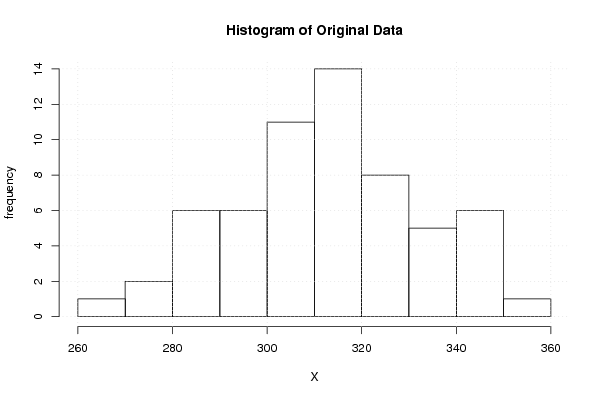
296.95 296.84 287.54 287.81 283.99 275.79 269.52 278.35 283.43 289.46 282.30 293.55 304.78 300.99 315.29 316.21 331.79 329.38 317.27 317.98 340.28 339.21 336.71 340.11 347.72 328.68 303.05 299.83 320.04 317.94 303.31 308.85 319.19 314.52 312.39 315.77 320.23 309.45 296.54 297.28 301.39 306.68 305.91 314.76 323.34 341.58 330.12 318.16 317.84 325.39 327.56 329.77 333.29 346.10 358.00 344.82 313.30 301.26 306.38 319.31 | |||||||||||||||||||||||||||||||||||||
Tables (Output of Computation) | |||||||||||||||||||||||||||||||||||||
| |||||||||||||||||||||||||||||||||||||
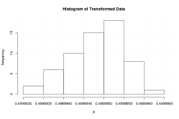
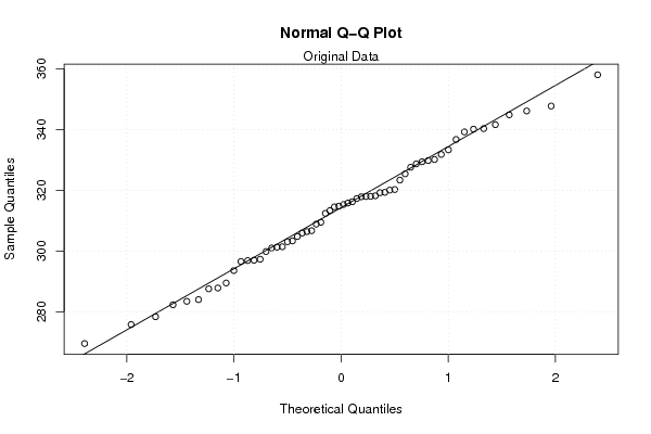
Figures (Output of Computation) | |||||||||||||||||||||||||||||||||||||
Input Parameters & R Code | |||||||||||||||||||||||||||||||||||||
| Parameters (Session): | |||||||||||||||||||||||||||||||||||||
| Parameters (R input): | |||||||||||||||||||||||||||||||||||||
| R code (references can be found in the software module): | |||||||||||||||||||||||||||||||||||||
n <- length(x) | |||||||||||||||||||||||||||||||||||||