Free Statistics
of Irreproducible Research!
Description of Statistical Computation | |||||||||||||||||||||||||||||||||||||||||||||||||||||
|---|---|---|---|---|---|---|---|---|---|---|---|---|---|---|---|---|---|---|---|---|---|---|---|---|---|---|---|---|---|---|---|---|---|---|---|---|---|---|---|---|---|---|---|---|---|---|---|---|---|---|---|---|---|
| Author's title | |||||||||||||||||||||||||||||||||||||||||||||||||||||
| Author | *The author of this computation has been verified* | ||||||||||||||||||||||||||||||||||||||||||||||||||||
| R Software Module | rwasp_edauni.wasp | ||||||||||||||||||||||||||||||||||||||||||||||||||||
| Title produced by software | Univariate Explorative Data Analysis | ||||||||||||||||||||||||||||||||||||||||||||||||||||
| Date of computation | Wed, 15 Dec 2010 02:15:39 +0000 | ||||||||||||||||||||||||||||||||||||||||||||||||||||
| Cite this page as follows | Statistical Computations at FreeStatistics.org, Office for Research Development and Education, URL https://freestatistics.org/blog/index.php?v=date/2010/Dec/15/t12923792000zexcgw46n9f8hs.htm/, Retrieved Fri, 03 May 2024 06:02:31 +0000 | ||||||||||||||||||||||||||||||||||||||||||||||||||||
| Statistical Computations at FreeStatistics.org, Office for Research Development and Education, URL https://freestatistics.org/blog/index.php?pk=110303, Retrieved Fri, 03 May 2024 06:02:31 +0000 | |||||||||||||||||||||||||||||||||||||||||||||||||||||
| QR Codes: | |||||||||||||||||||||||||||||||||||||||||||||||||||||
|
| |||||||||||||||||||||||||||||||||||||||||||||||||||||
| Original text written by user: | |||||||||||||||||||||||||||||||||||||||||||||||||||||
| IsPrivate? | No (this computation is public) | ||||||||||||||||||||||||||||||||||||||||||||||||||||
| User-defined keywords | |||||||||||||||||||||||||||||||||||||||||||||||||||||
| Estimated Impact | 164 | ||||||||||||||||||||||||||||||||||||||||||||||||||||
Tree of Dependent Computations | |||||||||||||||||||||||||||||||||||||||||||||||||||||
| Family? (F = Feedback message, R = changed R code, M = changed R Module, P = changed Parameters, D = changed Data) | |||||||||||||||||||||||||||||||||||||||||||||||||||||
| - [Recursive Partitioning (Regression Trees)] [] [2010-12-05 18:59:57] [b98453cac15ba1066b407e146608df68] - PD [Recursive Partitioning (Regression Trees)] [Recursive Partiti...] [2010-12-14 19:55:28] [c2a9e95daa10045f9fd6252038bcb219] - RMPD [Kendall tau Correlation Matrix] [Sleep] [2010-12-14 21:45:48] [c2a9e95daa10045f9fd6252038bcb219] - RMPD [Univariate Explorative Data Analysis] [EDA-weight] [2010-12-15 00:55:49] [d672a41e0af7ff107c03f1d65e47fd32] - D [Univariate Explorative Data Analysis] [EDA-lichaamsgewicht] [2010-12-15 01:05:39] [d672a41e0af7ff107c03f1d65e47fd32] - D [Univariate Explorative Data Analysis] [EDA-hersengewicht] [2010-12-15 01:08:41] [d672a41e0af7ff107c03f1d65e47fd32] - RMPD [Kendall tau Correlation Matrix] [Pearson Correlati...] [2010-12-15 01:18:33] [c2a9e95daa10045f9fd6252038bcb219] - RM D [Univariate Explorative Data Analysis] [] [2010-12-15 02:15:39] [c6b3e187a4a1689d42fffda4bc860ab5] [Current] | |||||||||||||||||||||||||||||||||||||||||||||||||||||
| Feedback Forum | |||||||||||||||||||||||||||||||||||||||||||||||||||||
Post a new message | |||||||||||||||||||||||||||||||||||||||||||||||||||||
Dataset | |||||||||||||||||||||||||||||||||||||||||||||||||||||
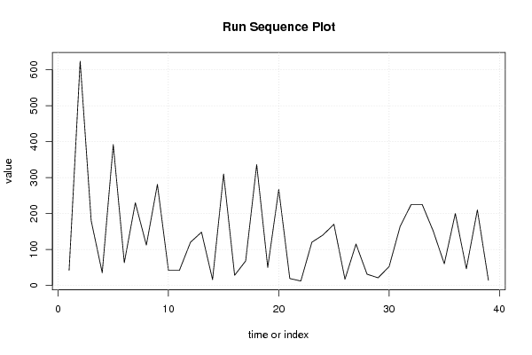
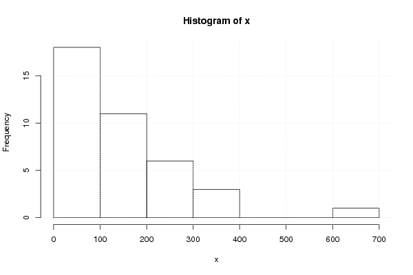
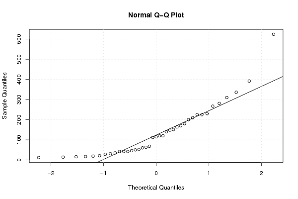
| Dataseries X: | |||||||||||||||||||||||||||||||||||||||||||||||||||||
42 624 180 35 392 63 230 112 281 42 42 120 148 16 310 28 68 336 50 267 19 12 120 140 170 17 115 31 21 52 164 225 225 151 60 200 46 210 14 | |||||||||||||||||||||||||||||||||||||||||||||||||||||
Tables (Output of Computation) | |||||||||||||||||||||||||||||||||||||||||||||||||||||
| |||||||||||||||||||||||||||||||||||||||||||||||||||||
Figures (Output of Computation) | |||||||||||||||||||||||||||||||||||||||||||||||||||||
Input Parameters & R Code | |||||||||||||||||||||||||||||||||||||||||||||||||||||
| Parameters (Session): | |||||||||||||||||||||||||||||||||||||||||||||||||||||
| par1 = 1 ; par2 = Do not include Seasonal Dummies ; par3 = No Linear Trend ; | |||||||||||||||||||||||||||||||||||||||||||||||||||||
| Parameters (R input): | |||||||||||||||||||||||||||||||||||||||||||||||||||||
| par1 = 0 ; par2 = 0 ; | |||||||||||||||||||||||||||||||||||||||||||||||||||||
| R code (references can be found in the software module): | |||||||||||||||||||||||||||||||||||||||||||||||||||||
par1 <- as.numeric(par1) | |||||||||||||||||||||||||||||||||||||||||||||||||||||