Free Statistics
of Irreproducible Research!
Description of Statistical Computation | |||||||||||||||||||||||||||||||||||||||||||||||||||||
|---|---|---|---|---|---|---|---|---|---|---|---|---|---|---|---|---|---|---|---|---|---|---|---|---|---|---|---|---|---|---|---|---|---|---|---|---|---|---|---|---|---|---|---|---|---|---|---|---|---|---|---|---|---|
| Author's title | |||||||||||||||||||||||||||||||||||||||||||||||||||||
| Author | *The author of this computation has been verified* | ||||||||||||||||||||||||||||||||||||||||||||||||||||
| R Software Module | rwasp_edauni.wasp | ||||||||||||||||||||||||||||||||||||||||||||||||||||
| Title produced by software | Univariate Explorative Data Analysis | ||||||||||||||||||||||||||||||||||||||||||||||||||||
| Date of computation | Wed, 15 Dec 2010 02:13:50 +0000 | ||||||||||||||||||||||||||||||||||||||||||||||||||||
| Cite this page as follows | Statistical Computations at FreeStatistics.org, Office for Research Development and Education, URL https://freestatistics.org/blog/index.php?v=date/2010/Dec/15/t1292379093grg1r4031x0h7tf.htm/, Retrieved Fri, 03 May 2024 06:47:35 +0000 | ||||||||||||||||||||||||||||||||||||||||||||||||||||
| Statistical Computations at FreeStatistics.org, Office for Research Development and Education, URL https://freestatistics.org/blog/index.php?pk=110301, Retrieved Fri, 03 May 2024 06:47:35 +0000 | |||||||||||||||||||||||||||||||||||||||||||||||||||||
| QR Codes: | |||||||||||||||||||||||||||||||||||||||||||||||||||||
|
| |||||||||||||||||||||||||||||||||||||||||||||||||||||
| Original text written by user: | |||||||||||||||||||||||||||||||||||||||||||||||||||||
| IsPrivate? | No (this computation is public) | ||||||||||||||||||||||||||||||||||||||||||||||||||||
| User-defined keywords | |||||||||||||||||||||||||||||||||||||||||||||||||||||
| Estimated Impact | 153 | ||||||||||||||||||||||||||||||||||||||||||||||||||||
Tree of Dependent Computations | |||||||||||||||||||||||||||||||||||||||||||||||||||||
| Family? (F = Feedback message, R = changed R code, M = changed R Module, P = changed Parameters, D = changed Data) | |||||||||||||||||||||||||||||||||||||||||||||||||||||
| - [Recursive Partitioning (Regression Trees)] [] [2010-12-05 18:59:57] [b98453cac15ba1066b407e146608df68] - PD [Recursive Partitioning (Regression Trees)] [Recursive Partiti...] [2010-12-14 19:55:28] [c2a9e95daa10045f9fd6252038bcb219] - RMPD [Kendall tau Correlation Matrix] [Sleep] [2010-12-14 21:45:48] [c2a9e95daa10045f9fd6252038bcb219] - RMPD [Univariate Explorative Data Analysis] [EDA-weight] [2010-12-15 00:55:49] [d672a41e0af7ff107c03f1d65e47fd32] - D [Univariate Explorative Data Analysis] [EDA-lichaamsgewicht] [2010-12-15 01:05:39] [d672a41e0af7ff107c03f1d65e47fd32] - D [Univariate Explorative Data Analysis] [EDA-hersengewicht] [2010-12-15 01:08:41] [d672a41e0af7ff107c03f1d65e47fd32] - RMPD [Kendall tau Correlation Matrix] [Pearson Correlati...] [2010-12-15 01:18:33] [c2a9e95daa10045f9fd6252038bcb219] - RM D [Univariate Explorative Data Analysis] [] [2010-12-15 02:13:50] [c6b3e187a4a1689d42fffda4bc860ab5] [Current] | |||||||||||||||||||||||||||||||||||||||||||||||||||||
| Feedback Forum | |||||||||||||||||||||||||||||||||||||||||||||||||||||
Post a new message | |||||||||||||||||||||||||||||||||||||||||||||||||||||
Dataset | |||||||||||||||||||||||||||||||||||||||||||||||||||||
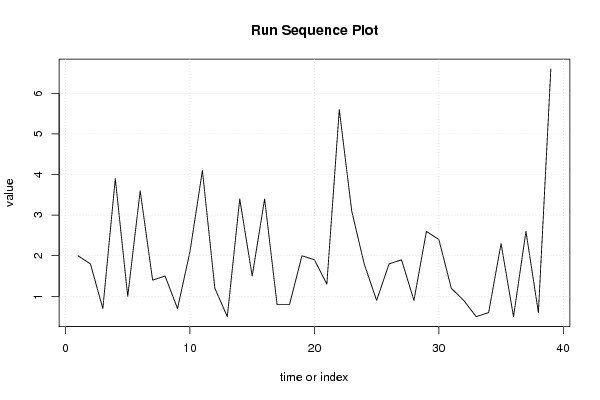
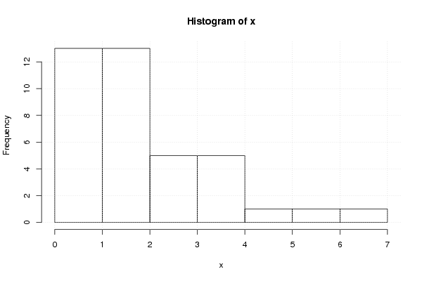
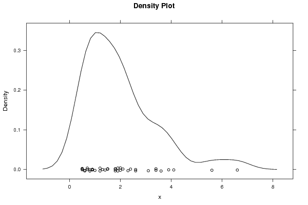
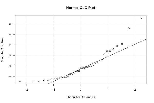
| Dataseries X: | |||||||||||||||||||||||||||||||||||||||||||||||||||||
2 1.8 0.7 3.9 1 3.6 1.4 1.5 0.7 2.1 4.1 1.2 0.5 3.4 1.5 3.4 0.8 0.8 2 1.9 1.3 5.6 3.1 1.8 0.9 1.8 1.9 0.9 2.6 2.4 1.2 0.9 0.5 0.6 2.3 0.5 2.6 0.6 6.6 | |||||||||||||||||||||||||||||||||||||||||||||||||||||
Tables (Output of Computation) | |||||||||||||||||||||||||||||||||||||||||||||||||||||
| |||||||||||||||||||||||||||||||||||||||||||||||||||||
Figures (Output of Computation) | |||||||||||||||||||||||||||||||||||||||||||||||||||||
Input Parameters & R Code | |||||||||||||||||||||||||||||||||||||||||||||||||||||
| Parameters (Session): | |||||||||||||||||||||||||||||||||||||||||||||||||||||
| par1 = 1 ; par2 = Do not include Seasonal Dummies ; par3 = No Linear Trend ; | |||||||||||||||||||||||||||||||||||||||||||||||||||||
| Parameters (R input): | |||||||||||||||||||||||||||||||||||||||||||||||||||||
| par1 = 0 ; par2 = 0 ; | |||||||||||||||||||||||||||||||||||||||||||||||||||||
| R code (references can be found in the software module): | |||||||||||||||||||||||||||||||||||||||||||||||||||||
par1 <- as.numeric(par1) | |||||||||||||||||||||||||||||||||||||||||||||||||||||