Free Statistics
of Irreproducible Research!
Description of Statistical Computation | |||||||||||||||||||||||||||||||||||||||||||||||||||||||||||||
|---|---|---|---|---|---|---|---|---|---|---|---|---|---|---|---|---|---|---|---|---|---|---|---|---|---|---|---|---|---|---|---|---|---|---|---|---|---|---|---|---|---|---|---|---|---|---|---|---|---|---|---|---|---|---|---|---|---|---|---|---|---|
| Author's title | |||||||||||||||||||||||||||||||||||||||||||||||||||||||||||||
| Author | *The author of this computation has been verified* | ||||||||||||||||||||||||||||||||||||||||||||||||||||||||||||
| R Software Module | rwasp_regression_trees1.wasp | ||||||||||||||||||||||||||||||||||||||||||||||||||||||||||||
| Title produced by software | Recursive Partitioning (Regression Trees) | ||||||||||||||||||||||||||||||||||||||||||||||||||||||||||||
| Date of computation | Tue, 14 Dec 2010 20:06:16 +0000 | ||||||||||||||||||||||||||||||||||||||||||||||||||||||||||||
| Cite this page as follows | Statistical Computations at FreeStatistics.org, Office for Research Development and Education, URL https://freestatistics.org/blog/index.php?v=date/2010/Dec/14/t12923571548uupvb34aa99ht1.htm/, Retrieved Thu, 02 May 2024 23:05:21 +0000 | ||||||||||||||||||||||||||||||||||||||||||||||||||||||||||||
| Statistical Computations at FreeStatistics.org, Office for Research Development and Education, URL https://freestatistics.org/blog/index.php?pk=110124, Retrieved Thu, 02 May 2024 23:05:21 +0000 | |||||||||||||||||||||||||||||||||||||||||||||||||||||||||||||
| QR Codes: | |||||||||||||||||||||||||||||||||||||||||||||||||||||||||||||
|
| |||||||||||||||||||||||||||||||||||||||||||||||||||||||||||||
| Original text written by user: | |||||||||||||||||||||||||||||||||||||||||||||||||||||||||||||
| IsPrivate? | No (this computation is public) | ||||||||||||||||||||||||||||||||||||||||||||||||||||||||||||
| User-defined keywords | |||||||||||||||||||||||||||||||||||||||||||||||||||||||||||||
| Estimated Impact | 171 | ||||||||||||||||||||||||||||||||||||||||||||||||||||||||||||
Tree of Dependent Computations | |||||||||||||||||||||||||||||||||||||||||||||||||||||||||||||
| Family? (F = Feedback message, R = changed R code, M = changed R Module, P = changed Parameters, D = changed Data) | |||||||||||||||||||||||||||||||||||||||||||||||||||||||||||||
| - [Kendall tau Correlation Matrix] [] [2010-12-05 17:44:33] [b98453cac15ba1066b407e146608df68] - R PD [Kendall tau Correlation Matrix] [WS10 Pearson] [2010-12-11 15:52:20] [afe9379cca749d06b3d6872e02cc47ed] - PD [Kendall tau Correlation Matrix] [WS10 Pearson] [2010-12-13 13:35:44] [afe9379cca749d06b3d6872e02cc47ed] F RMPD [Recursive Partitioning (Regression Trees)] [workshop 10 3] [2010-12-14 20:06:16] [97dee3ad7274585c4a7ecb4c981cc7fb] [Current] - [Recursive Partitioning (Regression Trees)] [verbetering WS 10 3] [2010-12-17 15:58:28] [033eb2749a430605d9b2be7c4aac4a0c] - [Recursive Partitioning (Regression Trees)] [] [2010-12-21 21:01:55] [9b13650c94c5192ca5135ec8a1fa39f7] - [Recursive Partitioning (Regression Trees)] [] [2010-12-21 23:28:42] [dd4fe494cff2ee46c12b15bdc7b848ca] | |||||||||||||||||||||||||||||||||||||||||||||||||||||||||||||
| Feedback Forum | |||||||||||||||||||||||||||||||||||||||||||||||||||||||||||||
Post a new message | |||||||||||||||||||||||||||||||||||||||||||||||||||||||||||||
Dataset | |||||||||||||||||||||||||||||||||||||||||||||||||||||||||||||
| Dataseries X: | |||||||||||||||||||||||||||||||||||||||||||||||||||||||||||||
24 14 11 12 24 26 25 11 7 8 25 23 17 6 17 8 30 25 18 12 10 8 19 23 18 8 12 9 22 19 16 10 12 7 22 29 20 10 11 4 25 25 16 11 11 11 23 21 18 16 12 7 17 22 17 11 13 7 21 25 23 13 14 12 19 24 30 12 16 10 19 18 23 8 11 10 15 22 18 12 10 8 16 15 15 11 11 8 23 22 12 4 15 4 27 28 21 9 9 9 22 20 15 8 11 8 14 12 20 8 17 7 22 24 31 14 17 11 23 20 27 15 11 9 23 21 34 16 18 11 21 20 21 9 14 13 19 21 31 14 10 8 18 23 19 11 11 8 20 28 16 8 15 9 23 24 20 9 15 6 25 24 21 9 13 9 19 24 22 9 16 9 24 23 17 9 13 6 22 23 24 10 9 6 25 29 25 16 18 16 26 24 26 11 18 5 29 18 25 8 12 7 32 25 17 9 17 9 25 21 32 16 9 6 29 26 33 11 9 6 28 22 13 16 12 5 17 22 32 12 18 12 28 22 25 12 12 7 29 23 29 14 18 10 26 30 22 9 14 9 25 23 18 10 15 8 14 17 17 9 16 5 25 23 20 10 10 8 26 23 15 12 11 8 20 25 20 14 14 10 18 24 33 14 9 6 32 24 29 10 12 8 25 23 23 14 17 7 25 21 26 16 5 4 23 24 18 9 12 8 21 24 20 10 12 8 20 28 11 6 6 4 15 16 28 8 24 20 30 20 26 13 12 8 24 29 22 10 12 8 26 27 17 8 14 6 24 22 12 7 7 4 22 28 14 15 13 8 14 16 17 9 12 9 24 25 21 10 13 6 24 24 19 12 14 7 24 28 18 13 8 9 24 24 10 10 11 5 19 23 29 11 9 5 31 30 31 8 11 8 22 24 19 9 13 8 27 21 9 13 10 6 19 25 20 11 11 8 25 25 28 8 12 7 20 22 19 9 9 7 21 23 30 9 15 9 27 26 29 15 18 11 23 23 26 9 15 6 25 25 23 10 12 8 20 21 13 14 13 6 21 25 21 12 14 9 22 24 19 12 10 8 23 29 28 11 13 6 25 22 23 14 13 10 25 27 18 6 11 8 17 26 21 12 13 8 19 22 20 8 16 10 25 24 23 14 8 5 19 27 21 11 16 7 20 24 21 10 11 5 26 24 15 14 9 8 23 29 28 12 16 14 27 22 19 10 12 7 17 21 26 14 14 8 17 24 10 5 8 6 19 24 16 11 9 5 17 23 22 10 15 6 22 20 19 9 11 10 21 27 31 10 21 12 32 26 31 16 14 9 21 25 29 13 18 12 21 21 19 9 12 7 18 21 22 10 13 8 18 19 23 10 15 10 23 21 15 7 12 6 19 21 20 9 19 10 20 16 18 8 15 10 21 22 23 14 11 10 20 29 25 14 11 5 17 15 21 8 10 7 18 17 24 9 13 10 19 15 25 14 15 11 22 21 17 14 12 6 15 21 13 8 12 7 14 19 28 8 16 12 18 24 21 8 9 11 24 20 25 7 18 11 35 17 9 6 8 11 29 23 16 8 13 5 21 24 19 6 17 8 25 14 17 11 9 6 20 19 25 14 15 9 22 24 20 11 8 4 13 13 29 11 7 4 26 22 14 11 12 7 17 16 22 14 14 11 25 19 15 8 6 6 20 25 19 20 8 7 19 25 20 11 17 8 21 23 15 8 10 4 22 24 20 11 11 8 24 26 18 10 14 9 21 26 33 14 11 8 26 25 22 11 13 11 24 18 16 9 12 8 16 21 17 9 11 5 23 26 16 8 9 4 18 23 21 10 12 8 16 23 26 13 20 10 26 22 18 13 12 6 19 20 18 12 13 9 21 13 17 8 12 9 21 24 22 13 12 13 22 15 30 14 9 9 23 14 30 12 15 10 29 22 24 14 24 20 21 10 21 15 7 5 21 24 21 13 17 11 23 22 29 16 11 6 27 24 31 9 17 9 25 19 20 9 11 7 21 20 16 9 12 9 10 13 22 8 14 10 20 20 20 7 11 9 26 22 28 16 16 8 24 24 38 11 21 7 29 29 22 9 14 6 19 12 20 11 20 13 24 20 17 9 13 6 19 21 28 14 11 8 24 24 22 13 15 10 22 22 31 16 19 16 17 20 | |||||||||||||||||||||||||||||||||||||||||||||||||||||||||||||
Tables (Output of Computation) | |||||||||||||||||||||||||||||||||||||||||||||||||||||||||||||
| |||||||||||||||||||||||||||||||||||||||||||||||||||||||||||||
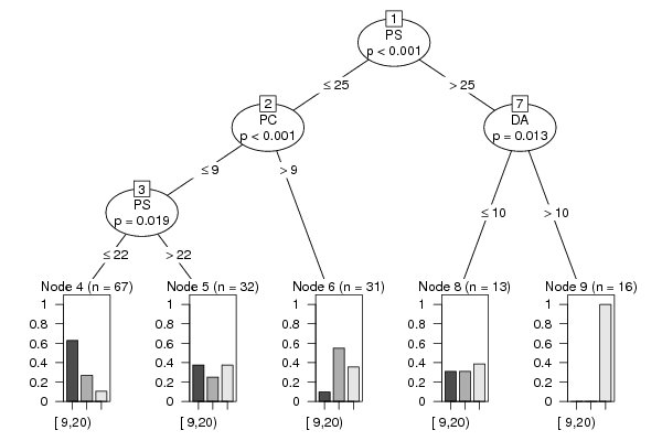
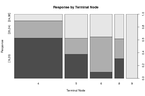
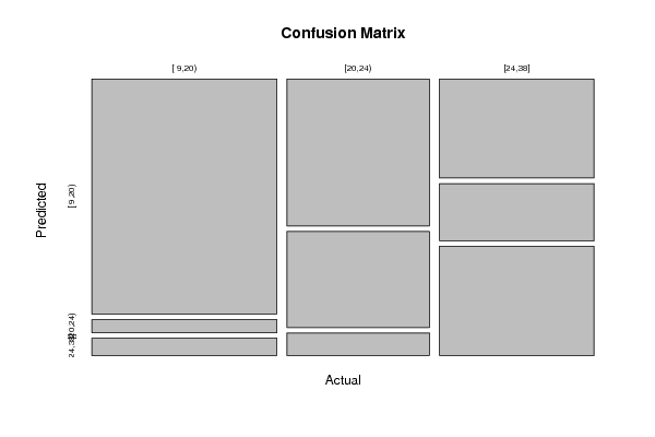
Figures (Output of Computation) | |||||||||||||||||||||||||||||||||||||||||||||||||||||||||||||
Input Parameters & R Code | |||||||||||||||||||||||||||||||||||||||||||||||||||||||||||||
| Parameters (Session): | |||||||||||||||||||||||||||||||||||||||||||||||||||||||||||||
| par1 = 1 ; par2 = none ; par3 = 3 ; par4 = no ; | |||||||||||||||||||||||||||||||||||||||||||||||||||||||||||||
| Parameters (R input): | |||||||||||||||||||||||||||||||||||||||||||||||||||||||||||||
| par1 = 1 ; par2 = quantiles ; par3 = 3 ; par4 = no ; | |||||||||||||||||||||||||||||||||||||||||||||||||||||||||||||
| R code (references can be found in the software module): | |||||||||||||||||||||||||||||||||||||||||||||||||||||||||||||
library(party) | |||||||||||||||||||||||||||||||||||||||||||||||||||||||||||||