Free Statistics
of Irreproducible Research!
Description of Statistical Computation | |||||||||||||||||||||||||||||||||||||||||||||||||||||||||||||
|---|---|---|---|---|---|---|---|---|---|---|---|---|---|---|---|---|---|---|---|---|---|---|---|---|---|---|---|---|---|---|---|---|---|---|---|---|---|---|---|---|---|---|---|---|---|---|---|---|---|---|---|---|---|---|---|---|---|---|---|---|---|
| Author's title | |||||||||||||||||||||||||||||||||||||||||||||||||||||||||||||
| Author | *The author of this computation has been verified* | ||||||||||||||||||||||||||||||||||||||||||||||||||||||||||||
| R Software Module | rwasp_linear_regression.wasp | ||||||||||||||||||||||||||||||||||||||||||||||||||||||||||||
| Title produced by software | Linear Regression Graphical Model Validation | ||||||||||||||||||||||||||||||||||||||||||||||||||||||||||||
| Date of computation | Tue, 14 Dec 2010 17:27:15 +0000 | ||||||||||||||||||||||||||||||||||||||||||||||||||||||||||||
| Cite this page as follows | Statistical Computations at FreeStatistics.org, Office for Research Development and Education, URL https://freestatistics.org/blog/index.php?v=date/2010/Dec/14/t1292347558dib8ujfc9cc9qbr.htm/, Retrieved Thu, 02 May 2024 19:45:32 +0000 | ||||||||||||||||||||||||||||||||||||||||||||||||||||||||||||
| Statistical Computations at FreeStatistics.org, Office for Research Development and Education, URL https://freestatistics.org/blog/index.php?pk=109926, Retrieved Thu, 02 May 2024 19:45:32 +0000 | |||||||||||||||||||||||||||||||||||||||||||||||||||||||||||||
| QR Codes: | |||||||||||||||||||||||||||||||||||||||||||||||||||||||||||||
|
| |||||||||||||||||||||||||||||||||||||||||||||||||||||||||||||
| Original text written by user: | |||||||||||||||||||||||||||||||||||||||||||||||||||||||||||||
| IsPrivate? | No (this computation is public) | ||||||||||||||||||||||||||||||||||||||||||||||||||||||||||||
| User-defined keywords | |||||||||||||||||||||||||||||||||||||||||||||||||||||||||||||
| Estimated Impact | 112 | ||||||||||||||||||||||||||||||||||||||||||||||||||||||||||||
Tree of Dependent Computations | |||||||||||||||||||||||||||||||||||||||||||||||||||||||||||||
| Family? (F = Feedback message, R = changed R code, M = changed R Module, P = changed Parameters, D = changed Data) | |||||||||||||||||||||||||||||||||||||||||||||||||||||||||||||
| - [Linear Regression Graphical Model Validation] [] [2010-12-14 17:27:15] [4dba6678eac10ee5c3460d144a14bd5c] [Current] | |||||||||||||||||||||||||||||||||||||||||||||||||||||||||||||
| Feedback Forum | |||||||||||||||||||||||||||||||||||||||||||||||||||||||||||||
Post a new message | |||||||||||||||||||||||||||||||||||||||||||||||||||||||||||||
Dataset | |||||||||||||||||||||||||||||||||||||||||||||||||||||||||||||
| Dataseries X: | |||||||||||||||||||||||||||||||||||||||||||||||||||||||||||||
32.50 37.00 38.00 39.50 39.50 39.50 39.50 38.00 36.00 36.00 36.00 37.00 38.00 38.00 38.00 38.00 38.00 36.00 36.00 36.00 36.00 35.00 36.00 35.00 33.85 31.56 28.48 33.45 35.93 35.07 34.16 33.95 35.63 35.68 34.15 31.72 31.19 28.95 28.82 30.61 30.00 31.00 31.66 31.91 31.11 30.41 29.84 29.24 29.69 30.15 30.76 30.62 30.52 29.97 28.75 29.25 29.31 28.77 28.10 25.43 25.64 27.27 28.24 28.81 27.62 27.14 27.33 27.76 28.29 29.54 30.81 27.23 22.95 15.44 12.62 12.85 15.44 13.47 11.58 15.09 14.91 14.85 15.21 16.08 18.66 17.73 18.31 18.64 19.42 20.03 21.36 20.27 19.53 19.85 18.92 17.24 17.16 16.77 16.22 17.88 17.44 16.53 15.50 15.52 14.47 13.80 13.98 16.27 17.98 17.83 19.45 21.04 20.03 20.01 19.64 18.52 19.59 20.09 19.82 21.09 22.64 22.11 20.42 18.58 18.24 16.87 18.64 27.17 33.69 35.92 32.30 27.34 24.96 20.52 19.86 20.82 21.24 20.20 21.42 21.69 21.86 23.23 22.47 19.52 18.82 19.00 18.92 20.24 20.94 22.38 21.76 21.35 21.90 21.69 20.34 19.41 19.08 20.05 20.35 20.27 19.94 19.07 17.87 18.01 17.51 18.15 16.70 14.51 15.00 14.78 14.66 16.38 17.88 19.07 19.65 18.38 17.46 17.71 18.10 17.16 17.99 18.53 18.55 19.87 19.74 18.42 17.30 18.03 18.23 17.44 17.99 19.04 18.88 19.07 21.36 23.57 21.25 20.45 21.32 21.96 23.99 24.90 23.71 25.39 25.17 22.21 20.99 19.72 20.83 19.17 19.63 19.93 19.79 21.26 20.17 18.32 16.71 16.06 15.02 15.44 14.86 13.66 14.08 13.36 14.95 14.39 12.85 11.28 12.47 12.01 14.66 17.34 17.75 17.89 20.07 21.26 23.88 22.64 24.97 26.08 27.18 29.35 29.89 25.74 28.78 31.83 29.77 31.22 33.88 33.08 34.40 28.46 29.58 29.61 27.24 27.41 28.64 27.60 26.45 27.47 25.88 22.21 19.67 19.33 19.67 20.74 24.42 26.27 27.02 25.52 26.94 28.38 29.67 28.85 26.27 29.42 32.94 35.87 33.55 28.25 28.14 30.72 30.76 31.59 28.29 30.33 31.09 32.15 34.27 34.74 36.76 36.69 40.28 38.02 40.69 44.94 45.95 53.13 48.46 43.33 46.84 47.97 54.31 53.04 49.83 56.26 58.70 64.97 65.57 62.37 58.30 59.43 65.51 61.63 62.90 69.69 70.94 70.96 74.41 73.05 63.87 58.88 59.37 62.03 54.57 59.26 60.56 63.97 63.46 67.48 74.18 72.39 79.93 86.20 94.62 91.73 92.95 95.35 105.56 112.57 125.39 133.93 133.44 116.61 103.90 76.65 57.44 41.02 41.74 39.16 47.98 49.79 59.16 69.68 64.09 71.06 69.46 75.82 78.08 74.30 | |||||||||||||||||||||||||||||||||||||||||||||||||||||||||||||
| Dataseries Y: | |||||||||||||||||||||||||||||||||||||||||||||||||||||||||||||
62348011 62715757 61647494 60391360 59778782 60008624 59608899 59446012 58297803 55842496 56668926 58047975 57891773 58156649 58809342 57803815 56994195 56310517 55016126 54079566 54190514 54556342 53982612 54949157 54696333 54057656 52235578 50937234 51782807 53723825 53304037 53226077 53081150 54797282 55385984 54251558 52769435 49818355 50742380 50965386 52665432 52875438 54658487 54505483 55159500 54898493 55266503 54461481 54576637 54927706 54649651 54848690 54467616 55744865 55024725 53346397 53805487 54216567 54233570 54193563 52957860 54427468 54646409 54220523 52783907 51325296 52354021 52217058 54096556 55780107 56257979 56572895 55524877 55534871 55038123 55142070 56320474 57091083 58227508 58880177 54854216 55210036 56137566 56307480 55612026 54915713 54174379 54847682 55652044 55352910 57916063 58713422 58106149 58301237 57839029 57913062 57132791 57212831 57574013 57885170 57602027 57266858 57691072 58847655 59201833 60885682 61344913 61592038 58696420 58217270 58619396 59049531 58970506 59007518 59525680 60417960 60500987 61071165 61831404 61474292 60916284 61173756 62077222 61800755 61233280 60404309 60508732 56960860 59508990 59849214 60667306 60878857 60697760 60386769 60642144 59242386 59065240 59257978 60251677 59554710 60594461 60549810 60795824 61204311 61272430 60435110 59785685 60145730 59017392 59259948 59724933 59711685 59973280 60771194 60482143 60802913 60618220 60973516 60258580 59555291 59741659 59457492 60063662 59885984 59897301 60361033 60424871 60812389 61069475 60890087 60798959 60337721 60781136 61096411 60697026 60589335 61197502 61695077 61869499 62190975 61785264 62304912 61557000 62358574 62363317 61504568 62457004 62588240 62983163 62642181 62840528 63230782 63160361 63557585 63408687 63261106 63261360 63580934 63667236 63338800 63809523 64166660 64615675 65188736 65122665 65479548 65465449 65991121 65337456 64567016 65011779 65891968 66242603 66760539 66614582 66427573 67648872 68016590 67899055 67761221 67224744 66948689 66819145 65829031 65915736 66034479 66877636 66701524 66937186 67258801 66936903 65495800 65303433 64261224 65774554 65664312 65708444 66214989 66194064 65383966 66417629 67041666 67073615 67735214 68247259 68040158 68665088 69491907 69501497 69945908 70501325 69239885 69158396 68689767 69352192 68419211 67731940 66173269 68112618 68286649 67814703 67716558 68069632 67653337 66803667 66897155 66698498 66176808 66750585 66606849 67068352 66793756 67330419 68739311 68837189 67179872 67722114 69312414 69844650 68764631 68761812 67951819 68570631 69025711 69694325 70598803 70831175 72088209 71775784 71755138 71699835 71665894 71341968 72940358 73397120 72367358 72987932 73603188 73264932 72898133 73163834 73468980 73788677 74078089 74190176 73840627 73692209 73736337 73289592 73355081 73851387 74146149 73641252 73599137 73426023 73485552 73046576 72938976 73972330 73624305 73340158 73650854 73327274 73106448 72784077 73040812 72959849 73198370 72722430 72333322 72846526 72199641 72975831 73652441 73360152 73786398 73899614 74062804 74235983 73659008 73967615 73977171 74685967 73476200 72537503 73553320 73390288 72590513 71551040 72074408 71875698 71995689 71611990 71800358 72708914 72245696 72653179 73111631 73165889 72891337 | |||||||||||||||||||||||||||||||||||||||||||||||||||||||||||||
Tables (Output of Computation) | |||||||||||||||||||||||||||||||||||||||||||||||||||||||||||||
| |||||||||||||||||||||||||||||||||||||||||||||||||||||||||||||
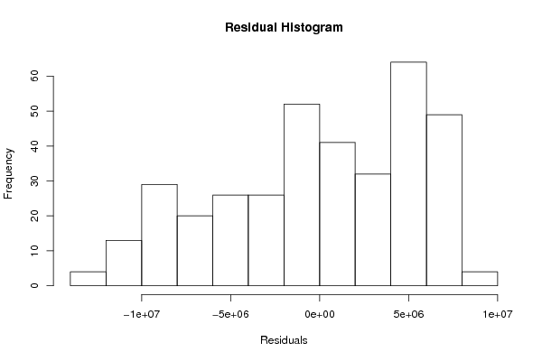
Figures (Output of Computation) | |||||||||||||||||||||||||||||||||||||||||||||||||||||||||||||
Input Parameters & R Code | |||||||||||||||||||||||||||||||||||||||||||||||||||||||||||||
| Parameters (Session): | |||||||||||||||||||||||||||||||||||||||||||||||||||||||||||||
| par1 = 0 ; | |||||||||||||||||||||||||||||||||||||||||||||||||||||||||||||
| Parameters (R input): | |||||||||||||||||||||||||||||||||||||||||||||||||||||||||||||
| par1 = 0 ; | |||||||||||||||||||||||||||||||||||||||||||||||||||||||||||||
| R code (references can be found in the software module): | |||||||||||||||||||||||||||||||||||||||||||||||||||||||||||||
par1 <- as.numeric(par1) | |||||||||||||||||||||||||||||||||||||||||||||||||||||||||||||