Repository of Reproducible Computations

Free Statistics

of Irreproducible Research!

Author's title

Author

*The author of this computation has been verified*

R Software Module

rwasp_autocorrelation.wasp

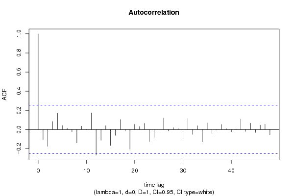
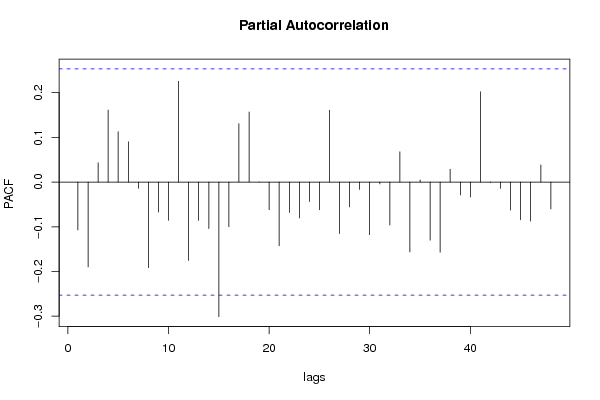
Title produced by software

(Partial) Autocorrelation Function

Date of computation

Tue, 14 Dec 2010 10:53:33 +0000

Cite this page as follows

Statistical Computations at FreeStatistics.org, Office for Research Development and Education, URL https://freestatistics.org/blog/index.php?v=date/2010/Dec/14/t1292323897gf03hjojujar07z.htm/, Retrieved Thu, 02 May 2024 17:22:49 +0000

Statistical Computations at FreeStatistics.org, Office for Research Development and Education, URL https://freestatistics.org/blog/index.php?pk=109389, Retrieved Thu, 02 May 2024 17:22:49 +0000

QR Codes:

Paste this QR Code to cite your computation.

Original text written by user:

IsPrivate?

No (this computation is public)

User-defined keywords

Estimated Impact

148

Family? (F = Feedback message, R = changed R code, M = changed R Module, P = changed Parameters, D = changed Data)

-     [(Partial) Autocorrelation Function] [Faillissementen V...] [2010-12-14 08:51:21] [13c73ac943380855a1c72833078e44d2]
-   P   [(Partial) Autocorrelation Function] [Faillissementen V...] [2010-12-14 09:09:28] [13c73ac943380855a1c72833078e44d2]
- RMP     [Spectral Analysis] [Faillissementen V...] [2010-12-14 09:27:52] [13c73ac943380855a1c72833078e44d2]
- RMPD      [(Partial) Autocorrelation Function] [Faillissementen W...] [2010-12-14 10:11:32] [049b50ae610f671f7417ed8e2d1295c1]
- RM          [Spectral Analysis] [Faillissementen W...] [2010-12-14 10:17:19] [049b50ae610f671f7417ed8e2d1295c1]
- RM D          [(Partial) Autocorrelation Function] [Faillissementen B...] [2010-12-14 10:47:49] [3074aa973ede76ac75d398946b01602f]
-                   [(Partial) Autocorrelation Function] [Faillissementen B...] [2010-12-14 10:53:33] [dcc54e7e6e8c80b7c45e040080afe6ab] [Current]

Feedback Forum

Post a new message

Dataseries X:

Download CSV

Histogram

Boxplots

Summary of computational transaction
Raw Input	view raw input (R code)
Raw Output	view raw output of R engine
Computing time	1 seconds
R Server	'Gwilym Jenkins' @ 72.249.127.135

\begin{tabular}{lllllllll}
\hline
Summary of computational transaction \tabularnewline
Raw Input & view raw input (R code)  \tabularnewline
Raw Output & view raw output of R engine  \tabularnewline
Computing time & 1 seconds \tabularnewline
R Server & 'Gwilym Jenkins' @ 72.249.127.135 \tabularnewline
\hline
\end{tabular}
%Source: https://freestatistics.org/blog/index.php?pk=109389&T=0

[TABLE]
[ROW][C]Summary of computational transaction[/C][/ROW]
[ROW][C]Raw Input[/C][C]view raw input (R code) [/C][/ROW]
[ROW][C]Raw Output[/C][C]view raw output of R engine [/C][/ROW]
[ROW][C]Computing time[/C][C]1 seconds[/C][/ROW]
[ROW][C]R Server[/C][C]'Gwilym Jenkins' @ 72.249.127.135[/C][/ROW]
[/TABLE]
Source: https://freestatistics.org/blog/index.php?pk=109389&T=0

Globally Unique Identifier (entire table): ba.freestatistics.org/blog/index.php?pk=109389&T=0

As an alternative you can also use a QR Code:

The GUIDs for individual cells are displayed in the table below:

Summary of computational transaction
Raw Input	view raw input (R code)
Raw Output	view raw output of R engine
Computing time	1 seconds
R Server	'Gwilym Jenkins' @ 72.249.127.135

Autocorrelation Function
Time lag k	ACF(k)	T-STAT	P-value
1	-0.106977	-0.8286	0.205297
2	-0.176109	-1.3641	0.088811
3	0.083821	0.6493	0.25932
4	0.171013	1.3247	0.095153
5	0.041602	0.3222	0.374194
6	0.012613	0.0977	0.461248
7	-0.025442	-0.1971	0.422219
8	-0.140043	-1.0848	0.141181
9	0.034171	0.2647	0.39608
10	-0.002047	-0.0159	0.493702
11	0.172273	1.3344	0.093555
12	-0.268097	-2.0767	0.021061
13	-0.112963	-0.875	0.192529
14	0.039608	0.3068	0.380029
15	-0.166949	-1.2932	0.100452
16	-0.060893	-0.4717	0.319434
17	0.10421	0.8072	0.211367
18	-0.014764	-0.1144	0.454667
19	-0.206993	-1.6034	0.057053
20	0.05519	0.4275	0.335273
21	0.030741	0.2381	0.406301
22	0.064431	0.4991	0.309775
23	-0.125236	-0.9701	0.167953
24	-0.082733	-0.6408	0.262031
25	-0.01488	-0.1153	0.454311
26	0.120024	0.9297	0.178125
27	-0.015339	-0.1188	0.452909
28	0.019929	0.1544	0.43892
29	0.012433	0.0963	0.4618
30	-0.097308	-0.7537	0.226976
31	0.114753	0.8889	0.188811
32	-0.050933	-0.3945	0.347295
33	0.038646	0.2994	0.382854
34	-0.129912	-1.0063	0.159158
35	0.069613	0.5392	0.295865
36	-0.041359	-0.3204	0.374902
37	-0.005804	-0.045	0.482145
38	0.053266	0.4126	0.340686
39	0.007974	0.0618	0.475478
40	-0.025289	-0.1959	0.42268
41	0.002214	0.0171	0.493188
42	0.109012	0.8444	0.200899
43	-0.019692	-0.1525	0.439638
44	0.066059	0.5117	0.305373
45	-0.029998	-0.2324	0.408524
46	0.04557	0.353	0.36267
47	0.055695	0.4314	0.333857
48	-0.05851	-0.4532	0.326014

\begin{tabular}{lllllllll}
\hline
Autocorrelation Function \tabularnewline
Time lag k & ACF(k) & T-STAT & P-value \tabularnewline
1 & -0.106977 & -0.8286 & 0.205297 \tabularnewline
2 & -0.176109 & -1.3641 & 0.088811 \tabularnewline
3 & 0.083821 & 0.6493 & 0.25932 \tabularnewline
4 & 0.171013 & 1.3247 & 0.095153 \tabularnewline
5 & 0.041602 & 0.3222 & 0.374194 \tabularnewline
6 & 0.012613 & 0.0977 & 0.461248 \tabularnewline
7 & -0.025442 & -0.1971 & 0.422219 \tabularnewline
8 & -0.140043 & -1.0848 & 0.141181 \tabularnewline
9 & 0.034171 & 0.2647 & 0.39608 \tabularnewline
10 & -0.002047 & -0.0159 & 0.493702 \tabularnewline
11 & 0.172273 & 1.3344 & 0.093555 \tabularnewline
12 & -0.268097 & -2.0767 & 0.021061 \tabularnewline
13 & -0.112963 & -0.875 & 0.192529 \tabularnewline
14 & 0.039608 & 0.3068 & 0.380029 \tabularnewline
15 & -0.166949 & -1.2932 & 0.100452 \tabularnewline
16 & -0.060893 & -0.4717 & 0.319434 \tabularnewline
17 & 0.10421 & 0.8072 & 0.211367 \tabularnewline
18 & -0.014764 & -0.1144 & 0.454667 \tabularnewline
19 & -0.206993 & -1.6034 & 0.057053 \tabularnewline
20 & 0.05519 & 0.4275 & 0.335273 \tabularnewline
21 & 0.030741 & 0.2381 & 0.406301 \tabularnewline
22 & 0.064431 & 0.4991 & 0.309775 \tabularnewline
23 & -0.125236 & -0.9701 & 0.167953 \tabularnewline
24 & -0.082733 & -0.6408 & 0.262031 \tabularnewline
25 & -0.01488 & -0.1153 & 0.454311 \tabularnewline
26 & 0.120024 & 0.9297 & 0.178125 \tabularnewline
27 & -0.015339 & -0.1188 & 0.452909 \tabularnewline
28 & 0.019929 & 0.1544 & 0.43892 \tabularnewline
29 & 0.012433 & 0.0963 & 0.4618 \tabularnewline
30 & -0.097308 & -0.7537 & 0.226976 \tabularnewline
31 & 0.114753 & 0.8889 & 0.188811 \tabularnewline
32 & -0.050933 & -0.3945 & 0.347295 \tabularnewline
33 & 0.038646 & 0.2994 & 0.382854 \tabularnewline
34 & -0.129912 & -1.0063 & 0.159158 \tabularnewline
35 & 0.069613 & 0.5392 & 0.295865 \tabularnewline
36 & -0.041359 & -0.3204 & 0.374902 \tabularnewline
37 & -0.005804 & -0.045 & 0.482145 \tabularnewline
38 & 0.053266 & 0.4126 & 0.340686 \tabularnewline
39 & 0.007974 & 0.0618 & 0.475478 \tabularnewline
40 & -0.025289 & -0.1959 & 0.42268 \tabularnewline
41 & 0.002214 & 0.0171 & 0.493188 \tabularnewline
42 & 0.109012 & 0.8444 & 0.200899 \tabularnewline
43 & -0.019692 & -0.1525 & 0.439638 \tabularnewline
44 & 0.066059 & 0.5117 & 0.305373 \tabularnewline
45 & -0.029998 & -0.2324 & 0.408524 \tabularnewline
46 & 0.04557 & 0.353 & 0.36267 \tabularnewline
47 & 0.055695 & 0.4314 & 0.333857 \tabularnewline
48 & -0.05851 & -0.4532 & 0.326014 \tabularnewline
\hline
\end{tabular}
%Source: https://freestatistics.org/blog/index.php?pk=109389&T=1

[TABLE]
[ROW][C]Autocorrelation Function[/C][/ROW]
[ROW][C]Time lag k[/C][C]ACF(k)[/C][C]T-STAT[/C][C]P-value[/C][/ROW]
[ROW][C]1[/C][C]-0.106977[/C][C]-0.8286[/C][C]0.205297[/C][/ROW]
[ROW][C]2[/C][C]-0.176109[/C][C]-1.3641[/C][C]0.088811[/C][/ROW]
[ROW][C]3[/C][C]0.083821[/C][C]0.6493[/C][C]0.25932[/C][/ROW]
[ROW][C]4[/C][C]0.171013[/C][C]1.3247[/C][C]0.095153[/C][/ROW]
[ROW][C]5[/C][C]0.041602[/C][C]0.3222[/C][C]0.374194[/C][/ROW]
[ROW][C]6[/C][C]0.012613[/C][C]0.0977[/C][C]0.461248[/C][/ROW]
[ROW][C]7[/C][C]-0.025442[/C][C]-0.1971[/C][C]0.422219[/C][/ROW]
[ROW][C]8[/C][C]-0.140043[/C][C]-1.0848[/C][C]0.141181[/C][/ROW]
[ROW][C]9[/C][C]0.034171[/C][C]0.2647[/C][C]0.39608[/C][/ROW]
[ROW][C]10[/C][C]-0.002047[/C][C]-0.0159[/C][C]0.493702[/C][/ROW]
[ROW][C]11[/C][C]0.172273[/C][C]1.3344[/C][C]0.093555[/C][/ROW]
[ROW][C]12[/C][C]-0.268097[/C][C]-2.0767[/C][C]0.021061[/C][/ROW]
[ROW][C]13[/C][C]-0.112963[/C][C]-0.875[/C][C]0.192529[/C][/ROW]
[ROW][C]14[/C][C]0.039608[/C][C]0.3068[/C][C]0.380029[/C][/ROW]
[ROW][C]15[/C][C]-0.166949[/C][C]-1.2932[/C][C]0.100452[/C][/ROW]
[ROW][C]16[/C][C]-0.060893[/C][C]-0.4717[/C][C]0.319434[/C][/ROW]
[ROW][C]17[/C][C]0.10421[/C][C]0.8072[/C][C]0.211367[/C][/ROW]
[ROW][C]18[/C][C]-0.014764[/C][C]-0.1144[/C][C]0.454667[/C][/ROW]
[ROW][C]19[/C][C]-0.206993[/C][C]-1.6034[/C][C]0.057053[/C][/ROW]
[ROW][C]20[/C][C]0.05519[/C][C]0.4275[/C][C]0.335273[/C][/ROW]
[ROW][C]21[/C][C]0.030741[/C][C]0.2381[/C][C]0.406301[/C][/ROW]
[ROW][C]22[/C][C]0.064431[/C][C]0.4991[/C][C]0.309775[/C][/ROW]
[ROW][C]23[/C][C]-0.125236[/C][C]-0.9701[/C][C]0.167953[/C][/ROW]
[ROW][C]24[/C][C]-0.082733[/C][C]-0.6408[/C][C]0.262031[/C][/ROW]
[ROW][C]25[/C][C]-0.01488[/C][C]-0.1153[/C][C]0.454311[/C][/ROW]
[ROW][C]26[/C][C]0.120024[/C][C]0.9297[/C][C]0.178125[/C][/ROW]
[ROW][C]27[/C][C]-0.015339[/C][C]-0.1188[/C][C]0.452909[/C][/ROW]
[ROW][C]28[/C][C]0.019929[/C][C]0.1544[/C][C]0.43892[/C][/ROW]
[ROW][C]29[/C][C]0.012433[/C][C]0.0963[/C][C]0.4618[/C][/ROW]
[ROW][C]30[/C][C]-0.097308[/C][C]-0.7537[/C][C]0.226976[/C][/ROW]
[ROW][C]31[/C][C]0.114753[/C][C]0.8889[/C][C]0.188811[/C][/ROW]
[ROW][C]32[/C][C]-0.050933[/C][C]-0.3945[/C][C]0.347295[/C][/ROW]
[ROW][C]33[/C][C]0.038646[/C][C]0.2994[/C][C]0.382854[/C][/ROW]
[ROW][C]34[/C][C]-0.129912[/C][C]-1.0063[/C][C]0.159158[/C][/ROW]
[ROW][C]35[/C][C]0.069613[/C][C]0.5392[/C][C]0.295865[/C][/ROW]
[ROW][C]36[/C][C]-0.041359[/C][C]-0.3204[/C][C]0.374902[/C][/ROW]
[ROW][C]37[/C][C]-0.005804[/C][C]-0.045[/C][C]0.482145[/C][/ROW]
[ROW][C]38[/C][C]0.053266[/C][C]0.4126[/C][C]0.340686[/C][/ROW]
[ROW][C]39[/C][C]0.007974[/C][C]0.0618[/C][C]0.475478[/C][/ROW]
[ROW][C]40[/C][C]-0.025289[/C][C]-0.1959[/C][C]0.42268[/C][/ROW]
[ROW][C]41[/C][C]0.002214[/C][C]0.0171[/C][C]0.493188[/C][/ROW]
[ROW][C]42[/C][C]0.109012[/C][C]0.8444[/C][C]0.200899[/C][/ROW]
[ROW][C]43[/C][C]-0.019692[/C][C]-0.1525[/C][C]0.439638[/C][/ROW]
[ROW][C]44[/C][C]0.066059[/C][C]0.5117[/C][C]0.305373[/C][/ROW]
[ROW][C]45[/C][C]-0.029998[/C][C]-0.2324[/C][C]0.408524[/C][/ROW]
[ROW][C]46[/C][C]0.04557[/C][C]0.353[/C][C]0.36267[/C][/ROW]
[ROW][C]47[/C][C]0.055695[/C][C]0.4314[/C][C]0.333857[/C][/ROW]
[ROW][C]48[/C][C]-0.05851[/C][C]-0.4532[/C][C]0.326014[/C][/ROW]
[/TABLE]
Source: https://freestatistics.org/blog/index.php?pk=109389&T=1

Globally Unique Identifier (entire table): ba.freestatistics.org/blog/index.php?pk=109389&T=1

As an alternative you can also use a QR Code:

The GUIDs for individual cells are displayed in the table below:

Autocorrelation Function
Time lag k	ACF(k)	T-STAT	P-value
1	-0.106977	-0.8286	0.205297
2	-0.176109	-1.3641	0.088811
3	0.083821	0.6493	0.25932
4	0.171013	1.3247	0.095153
5	0.041602	0.3222	0.374194
6	0.012613	0.0977	0.461248
7	-0.025442	-0.1971	0.422219
8	-0.140043	-1.0848	0.141181
9	0.034171	0.2647	0.39608
10	-0.002047	-0.0159	0.493702
11	0.172273	1.3344	0.093555
12	-0.268097	-2.0767	0.021061
13	-0.112963	-0.875	0.192529
14	0.039608	0.3068	0.380029
15	-0.166949	-1.2932	0.100452
16	-0.060893	-0.4717	0.319434
17	0.10421	0.8072	0.211367
18	-0.014764	-0.1144	0.454667
19	-0.206993	-1.6034	0.057053
20	0.05519	0.4275	0.335273
21	0.030741	0.2381	0.406301
22	0.064431	0.4991	0.309775
23	-0.125236	-0.9701	0.167953
24	-0.082733	-0.6408	0.262031
25	-0.01488	-0.1153	0.454311
26	0.120024	0.9297	0.178125
27	-0.015339	-0.1188	0.452909
28	0.019929	0.1544	0.43892
29	0.012433	0.0963	0.4618
30	-0.097308	-0.7537	0.226976
31	0.114753	0.8889	0.188811
32	-0.050933	-0.3945	0.347295
33	0.038646	0.2994	0.382854
34	-0.129912	-1.0063	0.159158
35	0.069613	0.5392	0.295865
36	-0.041359	-0.3204	0.374902
37	-0.005804	-0.045	0.482145
38	0.053266	0.4126	0.340686
39	0.007974	0.0618	0.475478
40	-0.025289	-0.1959	0.42268
41	0.002214	0.0171	0.493188
42	0.109012	0.8444	0.200899
43	-0.019692	-0.1525	0.439638
44	0.066059	0.5117	0.305373
45	-0.029998	-0.2324	0.408524
46	0.04557	0.353	0.36267
47	0.055695	0.4314	0.333857
48	-0.05851	-0.4532	0.326014

Partial Autocorrelation Function
Time lag k	PACF(k)	T-STAT	P-value
1	-0.106977	-0.8286	0.205297
2	-0.189724	-1.4696	0.073448
3	0.043139	0.3342	0.369713
4	0.161023	1.2473	0.108571
5	0.112582	0.8721	0.193327
6	0.090142	0.6982	0.243863
7	-0.013963	-0.1082	0.457117
8	-0.191576	-1.4839	0.07153
9	-0.067019	-0.5191	0.30279
10	-0.085418	-0.6616	0.255366
11	0.225505	1.7468	0.042899
12	-0.175634	-1.3605	0.089388
13	-0.085936	-0.6657	0.254091
14	-0.103976	-0.8054	0.211886
15	-0.301039	-2.3318	0.011542
16	-0.09975	-0.7727	0.221378
17	0.130669	1.0122	0.157764
18	0.156835	1.2148	0.114594
19	0.000202	0.0016	0.499378
20	-0.061896	-0.4794	0.316683
21	-0.142475	-1.1036	0.137085
22	-0.06822	-0.5284	0.299574
23	-0.080153	-0.6209	0.26852
24	-0.043514	-0.3371	0.368626
25	-0.062194	-0.4818	0.315867
26	0.160748	1.2451	0.108959
27	-0.115245	-0.8927	0.187797
28	-0.055577	-0.4305	0.334187
29	-0.016391	-0.127	0.449696
30	-0.117597	-0.9109	0.182995
31	-0.004091	-0.0317	0.487413
32	-0.096232	-0.7454	0.229467
33	0.067653	0.524	0.30109
34	-0.156373	-1.2113	0.115272
35	0.004642	0.036	0.485719
36	-0.13001	-1.0071	0.158976
37	-0.156783	-1.2144	0.114669
38	0.028913	0.224	0.411775
39	-0.02873	-0.2225	0.412323
40	-0.033243	-0.2575	0.398838
41	0.201982	1.5645	0.061474
42	-0.001132	-0.0088	0.496515
43	-0.014212	-0.1101	0.456356
44	-0.062577	-0.4847	0.314821
45	-0.084333	-0.6532	0.258049
46	-0.08734	-0.6765	0.250652
47	0.038419	0.2976	0.383521
48	-0.059975	-0.4646	0.321962

\begin{tabular}{lllllllll}
\hline
Partial Autocorrelation Function \tabularnewline
Time lag k & PACF(k) & T-STAT & P-value \tabularnewline
1 & -0.106977 & -0.8286 & 0.205297 \tabularnewline
2 & -0.189724 & -1.4696 & 0.073448 \tabularnewline
3 & 0.043139 & 0.3342 & 0.369713 \tabularnewline
4 & 0.161023 & 1.2473 & 0.108571 \tabularnewline
5 & 0.112582 & 0.8721 & 0.193327 \tabularnewline
6 & 0.090142 & 0.6982 & 0.243863 \tabularnewline
7 & -0.013963 & -0.1082 & 0.457117 \tabularnewline
8 & -0.191576 & -1.4839 & 0.07153 \tabularnewline
9 & -0.067019 & -0.5191 & 0.30279 \tabularnewline
10 & -0.085418 & -0.6616 & 0.255366 \tabularnewline
11 & 0.225505 & 1.7468 & 0.042899 \tabularnewline
12 & -0.175634 & -1.3605 & 0.089388 \tabularnewline
13 & -0.085936 & -0.6657 & 0.254091 \tabularnewline
14 & -0.103976 & -0.8054 & 0.211886 \tabularnewline
15 & -0.301039 & -2.3318 & 0.011542 \tabularnewline
16 & -0.09975 & -0.7727 & 0.221378 \tabularnewline
17 & 0.130669 & 1.0122 & 0.157764 \tabularnewline
18 & 0.156835 & 1.2148 & 0.114594 \tabularnewline
19 & 0.000202 & 0.0016 & 0.499378 \tabularnewline
20 & -0.061896 & -0.4794 & 0.316683 \tabularnewline
21 & -0.142475 & -1.1036 & 0.137085 \tabularnewline
22 & -0.06822 & -0.5284 & 0.299574 \tabularnewline
23 & -0.080153 & -0.6209 & 0.26852 \tabularnewline
24 & -0.043514 & -0.3371 & 0.368626 \tabularnewline
25 & -0.062194 & -0.4818 & 0.315867 \tabularnewline
26 & 0.160748 & 1.2451 & 0.108959 \tabularnewline
27 & -0.115245 & -0.8927 & 0.187797 \tabularnewline
28 & -0.055577 & -0.4305 & 0.334187 \tabularnewline
29 & -0.016391 & -0.127 & 0.449696 \tabularnewline
30 & -0.117597 & -0.9109 & 0.182995 \tabularnewline
31 & -0.004091 & -0.0317 & 0.487413 \tabularnewline
32 & -0.096232 & -0.7454 & 0.229467 \tabularnewline
33 & 0.067653 & 0.524 & 0.30109 \tabularnewline
34 & -0.156373 & -1.2113 & 0.115272 \tabularnewline
35 & 0.004642 & 0.036 & 0.485719 \tabularnewline
36 & -0.13001 & -1.0071 & 0.158976 \tabularnewline
37 & -0.156783 & -1.2144 & 0.114669 \tabularnewline
38 & 0.028913 & 0.224 & 0.411775 \tabularnewline
39 & -0.02873 & -0.2225 & 0.412323 \tabularnewline
40 & -0.033243 & -0.2575 & 0.398838 \tabularnewline
41 & 0.201982 & 1.5645 & 0.061474 \tabularnewline
42 & -0.001132 & -0.0088 & 0.496515 \tabularnewline
43 & -0.014212 & -0.1101 & 0.456356 \tabularnewline
44 & -0.062577 & -0.4847 & 0.314821 \tabularnewline
45 & -0.084333 & -0.6532 & 0.258049 \tabularnewline
46 & -0.08734 & -0.6765 & 0.250652 \tabularnewline
47 & 0.038419 & 0.2976 & 0.383521 \tabularnewline
48 & -0.059975 & -0.4646 & 0.321962 \tabularnewline
\hline
\end{tabular}
%Source: https://freestatistics.org/blog/index.php?pk=109389&T=2

[TABLE]
[ROW][C]Partial Autocorrelation Function[/C][/ROW]
[ROW][C]Time lag k[/C][C]PACF(k)[/C][C]T-STAT[/C][C]P-value[/C][/ROW]
[ROW][C]1[/C][C]-0.106977[/C][C]-0.8286[/C][C]0.205297[/C][/ROW]
[ROW][C]2[/C][C]-0.189724[/C][C]-1.4696[/C][C]0.073448[/C][/ROW]
[ROW][C]3[/C][C]0.043139[/C][C]0.3342[/C][C]0.369713[/C][/ROW]
[ROW][C]4[/C][C]0.161023[/C][C]1.2473[/C][C]0.108571[/C][/ROW]
[ROW][C]5[/C][C]0.112582[/C][C]0.8721[/C][C]0.193327[/C][/ROW]
[ROW][C]6[/C][C]0.090142[/C][C]0.6982[/C][C]0.243863[/C][/ROW]
[ROW][C]7[/C][C]-0.013963[/C][C]-0.1082[/C][C]0.457117[/C][/ROW]
[ROW][C]8[/C][C]-0.191576[/C][C]-1.4839[/C][C]0.07153[/C][/ROW]
[ROW][C]9[/C][C]-0.067019[/C][C]-0.5191[/C][C]0.30279[/C][/ROW]
[ROW][C]10[/C][C]-0.085418[/C][C]-0.6616[/C][C]0.255366[/C][/ROW]
[ROW][C]11[/C][C]0.225505[/C][C]1.7468[/C][C]0.042899[/C][/ROW]
[ROW][C]12[/C][C]-0.175634[/C][C]-1.3605[/C][C]0.089388[/C][/ROW]
[ROW][C]13[/C][C]-0.085936[/C][C]-0.6657[/C][C]0.254091[/C][/ROW]
[ROW][C]14[/C][C]-0.103976[/C][C]-0.8054[/C][C]0.211886[/C][/ROW]
[ROW][C]15[/C][C]-0.301039[/C][C]-2.3318[/C][C]0.011542[/C][/ROW]
[ROW][C]16[/C][C]-0.09975[/C][C]-0.7727[/C][C]0.221378[/C][/ROW]
[ROW][C]17[/C][C]0.130669[/C][C]1.0122[/C][C]0.157764[/C][/ROW]
[ROW][C]18[/C][C]0.156835[/C][C]1.2148[/C][C]0.114594[/C][/ROW]
[ROW][C]19[/C][C]0.000202[/C][C]0.0016[/C][C]0.499378[/C][/ROW]
[ROW][C]20[/C][C]-0.061896[/C][C]-0.4794[/C][C]0.316683[/C][/ROW]
[ROW][C]21[/C][C]-0.142475[/C][C]-1.1036[/C][C]0.137085[/C][/ROW]
[ROW][C]22[/C][C]-0.06822[/C][C]-0.5284[/C][C]0.299574[/C][/ROW]
[ROW][C]23[/C][C]-0.080153[/C][C]-0.6209[/C][C]0.26852[/C][/ROW]
[ROW][C]24[/C][C]-0.043514[/C][C]-0.3371[/C][C]0.368626[/C][/ROW]
[ROW][C]25[/C][C]-0.062194[/C][C]-0.4818[/C][C]0.315867[/C][/ROW]
[ROW][C]26[/C][C]0.160748[/C][C]1.2451[/C][C]0.108959[/C][/ROW]
[ROW][C]27[/C][C]-0.115245[/C][C]-0.8927[/C][C]0.187797[/C][/ROW]
[ROW][C]28[/C][C]-0.055577[/C][C]-0.4305[/C][C]0.334187[/C][/ROW]
[ROW][C]29[/C][C]-0.016391[/C][C]-0.127[/C][C]0.449696[/C][/ROW]
[ROW][C]30[/C][C]-0.117597[/C][C]-0.9109[/C][C]0.182995[/C][/ROW]
[ROW][C]31[/C][C]-0.004091[/C][C]-0.0317[/C][C]0.487413[/C][/ROW]
[ROW][C]32[/C][C]-0.096232[/C][C]-0.7454[/C][C]0.229467[/C][/ROW]
[ROW][C]33[/C][C]0.067653[/C][C]0.524[/C][C]0.30109[/C][/ROW]
[ROW][C]34[/C][C]-0.156373[/C][C]-1.2113[/C][C]0.115272[/C][/ROW]
[ROW][C]35[/C][C]0.004642[/C][C]0.036[/C][C]0.485719[/C][/ROW]
[ROW][C]36[/C][C]-0.13001[/C][C]-1.0071[/C][C]0.158976[/C][/ROW]
[ROW][C]37[/C][C]-0.156783[/C][C]-1.2144[/C][C]0.114669[/C][/ROW]
[ROW][C]38[/C][C]0.028913[/C][C]0.224[/C][C]0.411775[/C][/ROW]
[ROW][C]39[/C][C]-0.02873[/C][C]-0.2225[/C][C]0.412323[/C][/ROW]
[ROW][C]40[/C][C]-0.033243[/C][C]-0.2575[/C][C]0.398838[/C][/ROW]
[ROW][C]41[/C][C]0.201982[/C][C]1.5645[/C][C]0.061474[/C][/ROW]
[ROW][C]42[/C][C]-0.001132[/C][C]-0.0088[/C][C]0.496515[/C][/ROW]
[ROW][C]43[/C][C]-0.014212[/C][C]-0.1101[/C][C]0.456356[/C][/ROW]
[ROW][C]44[/C][C]-0.062577[/C][C]-0.4847[/C][C]0.314821[/C][/ROW]
[ROW][C]45[/C][C]-0.084333[/C][C]-0.6532[/C][C]0.258049[/C][/ROW]
[ROW][C]46[/C][C]-0.08734[/C][C]-0.6765[/C][C]0.250652[/C][/ROW]
[ROW][C]47[/C][C]0.038419[/C][C]0.2976[/C][C]0.383521[/C][/ROW]
[ROW][C]48[/C][C]-0.059975[/C][C]-0.4646[/C][C]0.321962[/C][/ROW]
[/TABLE]
Source: https://freestatistics.org/blog/index.php?pk=109389&T=2

Globally Unique Identifier (entire table): ba.freestatistics.org/blog/index.php?pk=109389&T=2

As an alternative you can also use a QR Code:

The GUIDs for individual cells are displayed in the table below:

Partial Autocorrelation Function
Time lag k	PACF(k)	T-STAT	P-value
1	-0.106977	-0.8286	0.205297
2	-0.189724	-1.4696	0.073448
3	0.043139	0.3342	0.369713
4	0.161023	1.2473	0.108571
5	0.112582	0.8721	0.193327
6	0.090142	0.6982	0.243863
7	-0.013963	-0.1082	0.457117
8	-0.191576	-1.4839	0.07153
9	-0.067019	-0.5191	0.30279
10	-0.085418	-0.6616	0.255366
11	0.225505	1.7468	0.042899
12	-0.175634	-1.3605	0.089388
13	-0.085936	-0.6657	0.254091
14	-0.103976	-0.8054	0.211886
15	-0.301039	-2.3318	0.011542
16	-0.09975	-0.7727	0.221378
17	0.130669	1.0122	0.157764
18	0.156835	1.2148	0.114594
19	0.000202	0.0016	0.499378
20	-0.061896	-0.4794	0.316683
21	-0.142475	-1.1036	0.137085
22	-0.06822	-0.5284	0.299574
23	-0.080153	-0.6209	0.26852
24	-0.043514	-0.3371	0.368626
25	-0.062194	-0.4818	0.315867
26	0.160748	1.2451	0.108959
27	-0.115245	-0.8927	0.187797
28	-0.055577	-0.4305	0.334187
29	-0.016391	-0.127	0.449696
30	-0.117597	-0.9109	0.182995
31	-0.004091	-0.0317	0.487413
32	-0.096232	-0.7454	0.229467
33	0.067653	0.524	0.30109
34	-0.156373	-1.2113	0.115272
35	0.004642	0.036	0.485719
36	-0.13001	-1.0071	0.158976
37	-0.156783	-1.2144	0.114669
38	0.028913	0.224	0.411775
39	-0.02873	-0.2225	0.412323
40	-0.033243	-0.2575	0.398838
41	0.201982	1.5645	0.061474
42	-0.001132	-0.0088	0.496515
43	-0.014212	-0.1101	0.456356
44	-0.062577	-0.4847	0.314821
45	-0.084333	-0.6532	0.258049
46	-0.08734	-0.6765	0.250652
47	0.038419	0.2976	0.383521
48	-0.059975	-0.4646	0.321962

Figure 1

PNG link

Postscript link

PDF link

Figure 2

PNG link

Postscript link

PDF link

Parameters (Session):

par1 = 12 ;

Parameters (R input):

par1 = 48 ; par2 = 1 ; par3 = 0 ; par4 = 1 ; par5 = 12 ; par6 = White Noise ; par7 = 0.95 ;

R code (references can be found in the software module):

if (par1 == 'Default') {
par1 = 10*log10(length(x))
} else {
par1 <- as.numeric(par1)
}
par2 <- as.numeric(par2)
par3 <- as.numeric(par3)
par4 <- as.numeric(par4)
par5 <- as.numeric(par5)
if (par6 == 'White Noise') par6 <- 'white' else par6 <- 'ma'
par7 <- as.numeric(par7)
if (par2 == 0) {
x <- log(x)
} else {
x <- (x ^ par2 - 1) / par2
}
if (par3 > 0) x <- diff(x,lag=1,difference=par3)
if (par4 > 0) x <- diff(x,lag=par5,difference=par4)
bitmap(file='pic1.png')
racf <- acf(x, par1, main='Autocorrelation', xlab='time lag', ylab='ACF', ci.type=par6, ci=par7, sub=paste('(lambda=',par2,', d=',par3,', D=',par4,', CI=', par7, ', CI type=',par6,')',sep=''))
dev.off()
bitmap(file='pic2.png')
rpacf <- pacf(x,par1,main='Partial Autocorrelation',xlab='lags',ylab='PACF')
dev.off()
(myacf <- c(racf$acf))
(mypacf <- c(rpacf$acf))
lengthx <- length(x)
sqrtn <- sqrt(lengthx)
load(file='createtable')
a<-table.start()
a<-table.row.start(a)
a<-table.element(a,'Autocorrelation Function',4,TRUE)
a<-table.row.end(a)
a<-table.row.start(a)
a<-table.element(a,'Time lag k',header=TRUE)
a<-table.element(a,hyperlink('basics.htm','ACF(k)','click here for more information about the Autocorrelation Function'),header=TRUE)
a<-table.element(a,'T-STAT',header=TRUE)
a<-table.element(a,'P-value',header=TRUE)
a<-table.row.end(a)
for (i in 2:(par1+1)) {
a<-table.row.start(a)
a<-table.element(a,i-1,header=TRUE)
a<-table.element(a,round(myacf[i],6))
mytstat <- myacf[i]*sqrtn
a<-table.element(a,round(mytstat,4))
a<-table.element(a,round(1-pt(abs(mytstat),lengthx),6))
a<-table.row.end(a)
}
a<-table.end(a)
table.save(a,file='mytable.tab')
a<-table.start()
a<-table.row.start(a)
a<-table.element(a,'Partial Autocorrelation Function',4,TRUE)
a<-table.row.end(a)
a<-table.row.start(a)
a<-table.element(a,'Time lag k',header=TRUE)
a<-table.element(a,hyperlink('basics.htm','PACF(k)','click here for more information about the Partial Autocorrelation Function'),header=TRUE)
a<-table.element(a,'T-STAT',header=TRUE)
a<-table.element(a,'P-value',header=TRUE)
a<-table.row.end(a)
for (i in 1:par1) {
a<-table.row.start(a)
a<-table.element(a,i,header=TRUE)
a<-table.element(a,round(mypacf[i],6))
mytstat <- mypacf[i]*sqrtn
a<-table.element(a,round(mytstat,4))
a<-table.element(a,round(1-pt(abs(mytstat),lengthx),6))
a<-table.row.end(a)
}
a<-table.end(a)
table.save(a,file='mytable1.tab')

Free Statistics

Description of Statistical Computation

Tree of Dependent Computations

Dataset

Tables (Output of Computation)

Figures (Output of Computation)

Input Parameters & R Code